The cloudy layers of modern-day programming

Recently, I’ve come to the realization that much of what we do in modern software development is not true software engineering. We spend the majority of our days trying to configure OpenSprocket 2.3.1 to work with NeoGidgetPro5, both of which were developed by two different third-party vendors and available as only as proprietary services in FoogleServiceCloud.
The name of this activity is, brilliantly summarized as VendorOps, from this blog post,
… the situation of putting together jigsaw puzzles with hammers, scissors, and tape, instead of having finely-crafted pieces that are designed to fit together.
I realize now that we need to label this properly. It’s “managed vendor stuff ops”, as a friend called it. When I read that off the window of my chat client a few minutes ago, it was like a bomb went off in my head. This is it! This explains so much!
It’s VendorOps. You are hired to tend the vendor’s stuff.
Instead of working on the core of the code and focusing on the performance of a self-contained application, developers are now forced to act as some kind of monstrous manual management layer between hundreds of various APIs, puzzling together whether Flark 2.3.5 on a T5.enormous instance will work with a Kappa function that sends data from ElephantStore in the us-polar-north-1 region to the APIFunctionFactoryTerminal in us-polar-south-2.
This kind of software development pattern is inevitable in our current development landscape, where everything is libraries developing on top of libraries, all of which, in the cloud, need network configuration as big cloud vendor network topologies determine the shape of our applications.
Although it’s something I’ve only thought about recently, top computer scientists have been recognizing this as a problem for at least the past ten years. Antirez, who wrote Redis, one of the most critical and elegant programs in use in high-volume production environments today, wrote a while back that,
[m]odern programming is becoming complex, uninteresting, full of layers that just need to be glued. It is losing most of its beauty. In that sense, most programming is no longer art nor high engineering (most programs written at big and small corporations are trivial: coders just need to understand certain ad-hoc abstractions, and write some logic and glue code).
Donald Knuth wrote,
“There’s the change that I’m really worried about: that the way a lot of programming goes today isn’t any fun because it’s just plugging in magic incantations — combine somebody else’s software and start it up. It doesn’t have much creativity. I’m worried that it’s becoming too boring because you don’t have a chance to do anything much new. Your kick comes out of seeing fun results coming out of the machine, but not the kind of kick that I always got by creating something new. The kick now is after you’ve done your boring work then all of a sudden you get a great image. But the work didn’t used to be boring.”
Although these concerns have been ongoing for at least the past ten years, they’ve exploded with the rise of the cloud. How did we get here? As Marianne Bellotti describes in “Kill It With Fire,” software development paradigms are a cycle, a continuous tradeoff between how cheap it is to process data on a single machine versus sending it over the network.
“Technology is, and probably always will be, an expensive element of any organization’s operational model. A great deal of advancement and market co-creation in technology can be understood as the interplay between hardware costs and network costs. Computers are data processors. They move data around and rearrange it into different formats and displays for us. All advancements with data processors come down to one of two things: either you make the machine faster or you make the pipes delivering data faster.”
We started with mainframe processing. Once we broke apart the mainframe into personal computers that were cheaper, we could write code locally. Then, our computers became even smaller and internet bandwidth became cheap, it made more sense to process and develop over the wire, particularly since much of our code was now tied up in web applications that lived in server farms. So, we sent everything to the cloud and started bundling development there.
Technology moves in cycles, and today, the cloud, is essentially, a big timeshare mainframe partitioned for millions of users. Aside from actual software concerns arising from this pattern, like the noisy neighbor problem, there is a larger overarching issue in that we are responsible for gluing together hundreds of tiny components and shipping networking logic to build a single app that is dependent on each cloud vendor’s implementations of specific technologies. From a historical context, it makes sense. As an engineer who just wants to build and ship substantial products, it makes me miserable.
Viberary
A specific example of this in the context of the recent work I’ve been doing on Viberary. Viberary is my ML side project that will eventually recommend books based not on genre or title, but vibe. The idea is pretty simple: return book recommendations based on semantic keywords that you put in. So you don’t put in “I want science fiction”, you’d put in “atmospheric, female lead, worldbuilding, funny” and get back a list of books.
For this project, I’m starting with the UCSD Goodreads Book Graph Dataset (in part because, ironically, in this age of APIs, Goodreads , or rather parent company Amazon, has decided to deprecate theirs. This dataset contains data from readers’ public shelves in scraped in late 2017. The project will eventually grow to include a trained deep learning model that learns embeddings both for the books and the semantic query and performs inference by matching the search term to the book’s embeddings and re-ranks them in a multistage process to give you the best recommendation for the text string you enter.
Here’s the architecture I’m envisioning:

None of that is important yet, though. What is important, as with any data project, is getting and analyzing the input data to understand if the data we have is valuable, useful for modeling, and if the architecture I’m envisioning even makes sense. Data visibility is critical at the first stages of the model, regardless of if you’re doing deep learning or using “traditional” tabular data methods.
Looking at the input data, the main book metadata dataset is ~2.3 million rows, which ends up being ~2GB.~ edit: it was 2 GB compressed, 10GB uncompressed JSON.
What I’d like to do with this data is:
- Read it into a persistent data store since I’ll want to continue to work with it again for feature selection, modeling, and fine-tuning any resulting models
- Work with a part or all of the data in-memory to profile it, visualize it, and then persist those artifacts (notebooks, images) for reference as I evaluate the data and refer back to it throughout the modeling process
My requirements mean that eventually I will need this project reliably in production on a server somewhere, particularly if I’m looking to do training and inference with GPUs, and even more so if I want to make Viberary a web app that people can use interactively. So it makes sense to start working with it in the cloud.
Since I’ve used AWS extensively before, I decided to switch to GCP for this particular project - what’s a side project if you can’t learn to break a bunch of new stuff?
The easiest/most common way to store data in GCP is BigQuery. There are multiple ways to work with BigQuery: the UI, the Cloud CLI, and the Cloud Shell. For the sake of brevity, I decided to go with local file upload from the original json file I had, and read it into a BigQuery table.
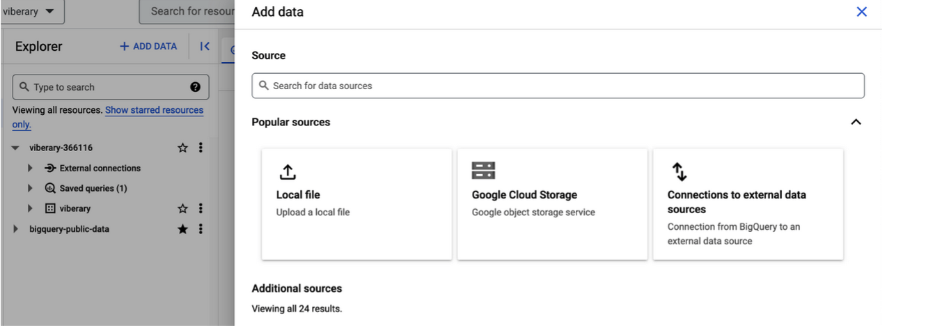
When you create a table in BigQuery, one of the things you can do is open that query directly in a Colab Notebook. Colab notebooks are Google’s proprietary implementation of Jupyter Notebook’s and are quickly becoming the lingua franca for exploring datasets and generating Stable Diffusion images since they’re free and tied to your Google account.
Spinning up a notebook generates a job that connects to BigQuery and runs that same query as you did directly in BigQuery, along with pre-populated boilerplate code to connect to the BigQuery job.The next cell renders this code as a pandas DataFrame using to_dataframe().
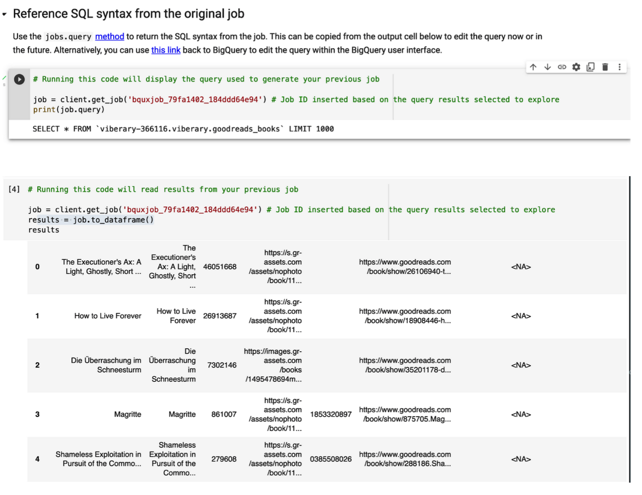
And now I can explore it. But this is just a sample of 1000 rows. Now what if I want to work with all my data in-memory? I run SELECT * FROM viberary-366116.viberary.goodreads_booksfrom mytable and the bigquery client tries very hard to run the query and send it in-memory to my machine, maxing out on RAM.
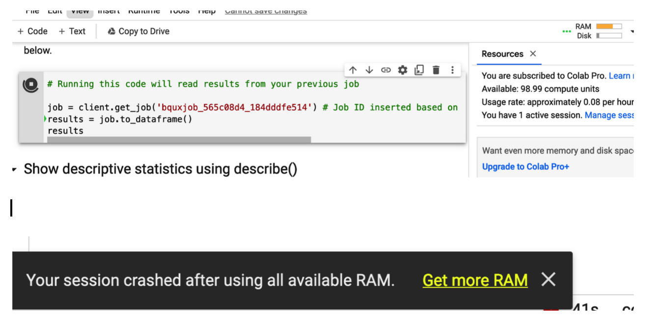
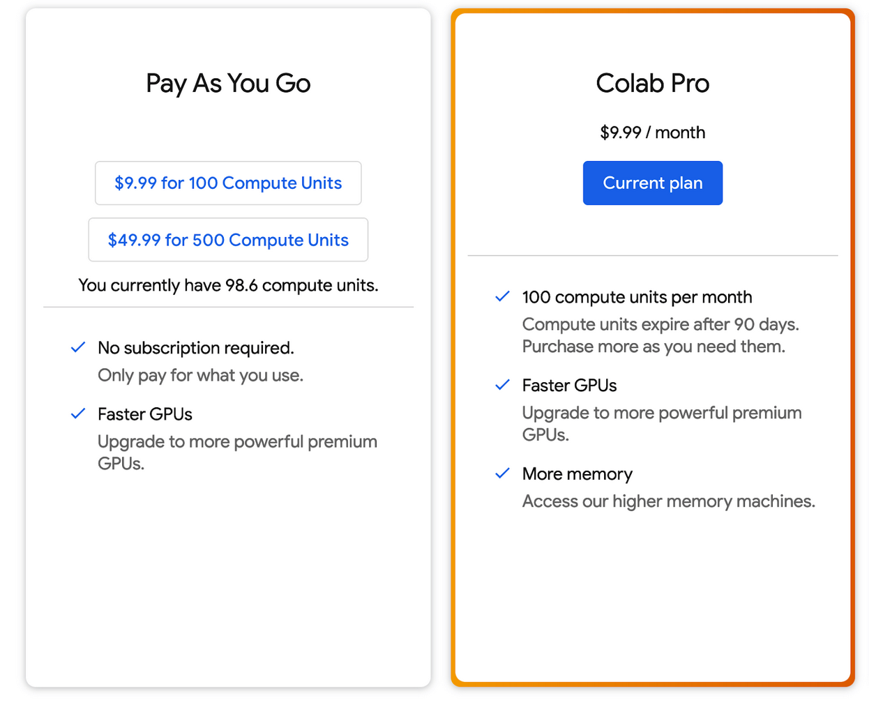
Then the notebook crashes. It helpfully offers me to upgrade to Colab Pro, even though I’m already running it.
What are my next options here? I could try:
\
- Sampling the data several times at random to get a general idea of its shape and properties \
- Going with a larger amount of RAM or \
- Use a distributed computation engine like Spark or Dask to work with it or \
- Figuring out what’s going on and tune processing, possibly with chunks
1-3 don’t entirely make sense to me yet, because based purely on vibes and my past experience (aka ghost knowledge),you should be able to read at least 1 million rows into memory with Pandas. The real constraint is how much RAM you have on your machine, but there are also soft constraints for the way Pandas renders Python objects into memory that make it difficult to deal with large datasets.

So what’s actually going on here? How do I profile the memory of a Notebook that I kicked off from a BigQuery job? Where do I even start trying to understand how to solve this problem? And how do I finally get to my data?
It makes sense to start at the beginning to understand what’s going on in my program.
Understanding the System
In System Performance, a great book I very strongly recommend everyone working even remotely close to production environments read, Brendan Gregg writes,
“Systems performance studies the performance of an entire computer system, including all the major software and hardware components. Anything in the data path, from storage devices to application software, is included, because it can affect performance. For distributed systems, this means multiple servers and applications. If you don’t have a diagram of your environment showing the data path, find one or draw it yourself: this will help you understand the relationships between components and ensure that you don’t overlook entire areas.”
The core of performance is looking at your code and its relationship to the machine it runs on. In the past, in the individual computing days, the machine and the code used to be symbiotic and it was easier to understand what was happening.
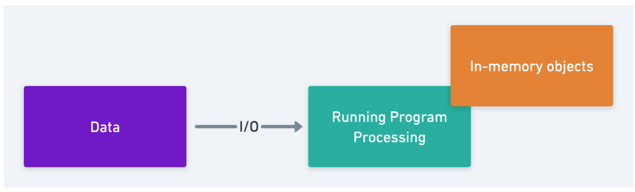
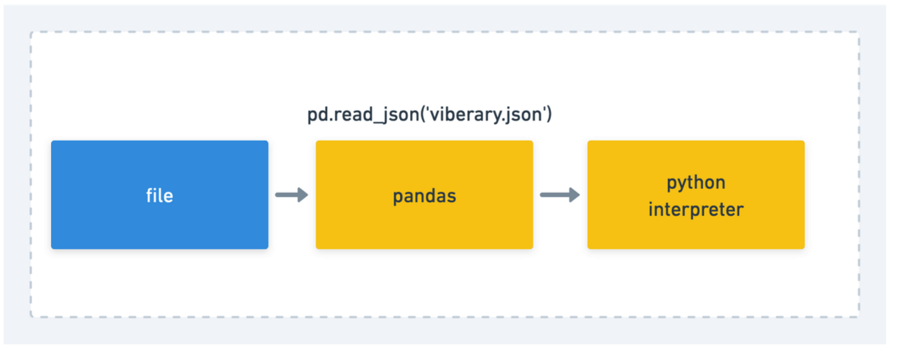
So, if we are working with plain vanilla Python, our system diagram would look something like this,
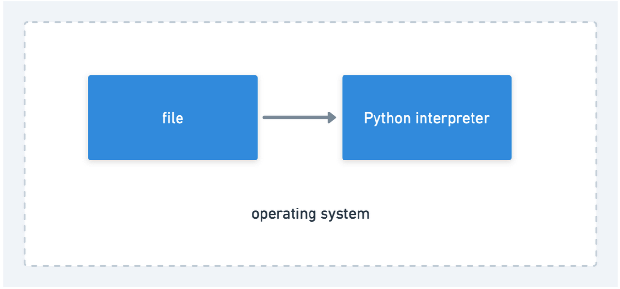
In “traditional” programming, there are several important metrics to look at for program performance:
- I/O throughput between the program and the data source
- The program’s CPU usage and
- the program’s memory footprint as it runs
When we profile, we want to understand where the issue is. We can look at this either from the operating system or the program level. In “Systems Performance”, Gregg covers a couple of high-level systems checks you can perform immediately to see what’s up.
Uptime \
dmesg | tail \
vmstat 1 \
mpstat -P ALL 1 \
pidstat 1 \
iostat -xz 1 \
free -m \
sar -n DEV 1 \
sar -n TCP,ETCP 1 \
top
Since we’re not as concerned about the interplay of programs as what’s going on immediately in our Python data processing application, we can take a look at these, but we want to profile at the program level.
When we profile standard Python programs, we can wrap our code in profiling code that will tell us how long each function call takes. The profiler tells us, on the command line, what the processing footprint of each method is. We can then also see how much memory is taken up by what we’re processing using something like memory-profiler.
import cProfile
import re

myfile = "goodreads_books.json"

def process_file(my_file):
   with open(my_file, "rb") as file:
       for line in file:
           do_work(line)

cProfile.run("process_file(myfile)")
If we don’t use Pandas, we’ll have to write a lot of custom functionality to convert our data into a DataFrame-like structure we can iterate over. But, it easier to reason about them individually it was a different programming paradigm. as described in this post about why MIT switched from Scheme to Python,
Costanza asked Sussman why MIT had switched away from Scheme for their introductory programming course, 6.001. This was a gem. He said that the reason that happened was because engineering in 1980 was not what it was in the mid-90s or in 2000. In 1980, good programmers spent a lot of time thinking, and then produced spare code that they thought should work. Code ran close to the metal, even Scheme — it was understandable all the way down. Like a resistor, where you could read the bands and know the power rating and the tolerance and the resistance and V=IR and that’s all there was to know. 6.001 had been conceived to teach engineers how to take small parts that they understood entirely and use simple techniques to compose them into larger things that do what you want.
As we transitioned to the age of programs written in modern languages that are further away from the bottom of the stack and closer to making web requests, we lose some of that ability to create larger, more meaningful programs.
But programming now isn’t so much like that, said Sussman. Nowadays you muck around with incomprehensible or nonexistent man pages for software you don’t know who wrote. You have to do basic science on your libraries to see how they work, trying out different inputs and seeing how the code reacts. This is a fundamentally different job, and it needed a different course.
Fast forward to today, if I were writing this code locally in a “modern data science” way, I might have two components:
- Pandas running as a Python library in a Jupyter Notebook
- Connected to some kind of local data store like SQLite, or, more realistically, reading it directly from a CSV file.
In that case, my system diagram would look like this:
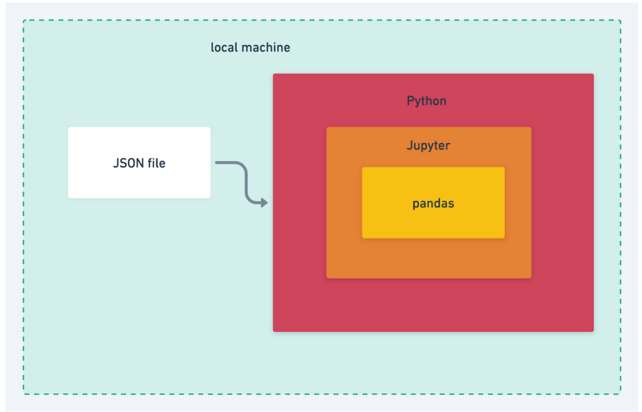
This is fairly simple, but we still need to dig in a bit more - what does it mean that pandas is running via Jupyter? How do notebooks work?
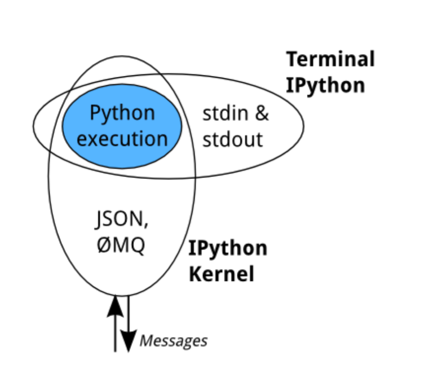
The main processing engine in Jupyter notebooks is the IPython kernel,a Python process that runs independently and interacts with Jupyter. It acts as the communication hub between the Python execution environment and other components, in our case, the front-end of the notebook where the user enters Python commands. (It can also connect to IPython in the terminal)
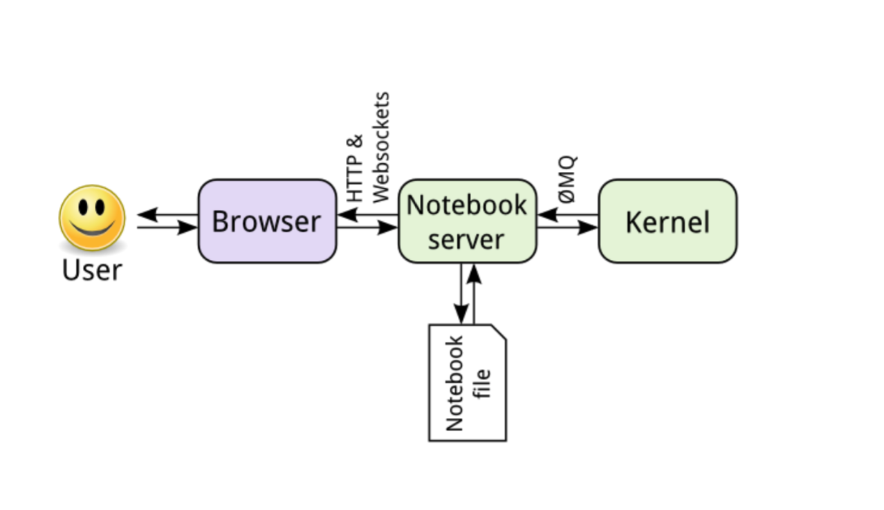
The notebook itself is based on a notebook server that acts as a central point of coordination between the code the user enters into the browser and the Python kernel. The kernel sends messages, via zeromq, to the iPython message handler, which passes it on to Python to run.
The notebook server is a communication hub. The browser, notebook file on disk, and kernel cannot talk to each other directly. They communicate through the notebook server. The notebook server, not the kernel, is responsible for saving and loading notebooks, so you can edit notebooks even if you don’t have the kernel for that language—you just won’t be able to run code. The kernel doesn’t know anything about the notebook document: it just gets sent cells of code to execute when the user runs them.
So what happens when we type in pd.read_json(‘data.json’) into a cell in the notebook? Due to the way the UI is designed, we generally think it’s something like this,
But the reality of the situation is something more like this:
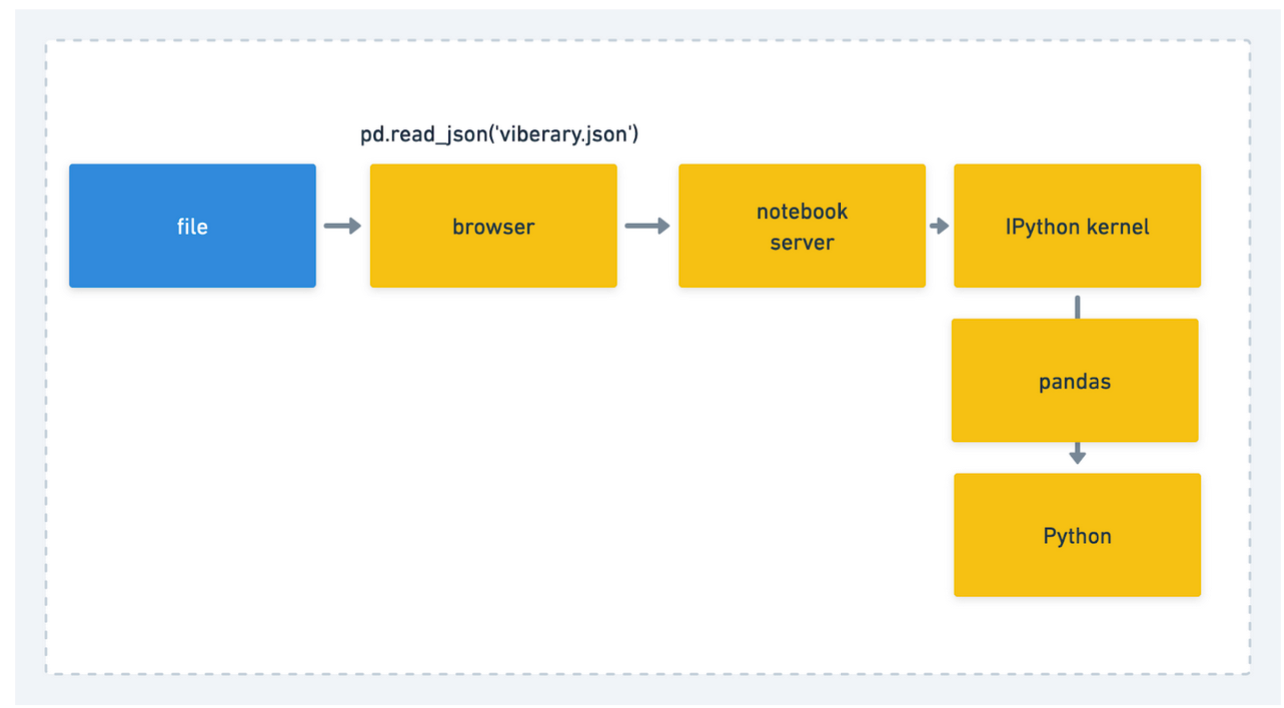
This becomes more complicated, because now, in addition to the performance of the program, we now need to account for pandas and the notebook server and the browser.
We can start with introspecting Pandas objects by reading the data from JSON. This will give us the size of each column in bytes. So we can see that if we read in a sample of 100 lines, it will take up
import pandas as pd

# reading in head -100 goodreads_books.json > goodreads_sample.json
pd.read_json('goodreads_sample.json',lines=True)

df.memory_usage(deep=True)

Index    128
uid       40
book      40
dtype: int64
By running info, we can see the total memory footprint: df.info()
<class 'pandas.core.frame.DataFrame'>

RangeIndex: 5 entries, 0 to 4

Data columns (total 2 columns):

 #   Column  Non-Null Count  Dtype
---  ------  --------------  -----
 0   uid     5 non-null      int64
 1   book    5 non-null      int64
dtypes: int64(2)
memory usage: 208.0 bytes
However, what this doesn’t tell us is how much memory we’ll consume when we’re running it on a larger sample - if we OOM in Pandas: these tools are not meant for profiling data-intensive flows.
Data processing (data pipelines, data workflows, batch jobs… terminology differs) is a whole different domain. For data processing, you are processing a lot of data together in one go. [Rereading above, the issue of latency and throughput and corresponding bottlenecks and how they differ between web and data processing is probably its own whole different discussion, so not going to discuss it any further in this braindump].Unlike web applications where all workers are handling similar workloads, data processing has much more sophisticated parallelism.
For example, you might have a main process that sets up the work, and the hands chunks to worker processes, and then reassembles. You might have multiple worker pools doing different things. You might have too many workers (https://pythonspeed.com/articles/concurrency-control/)! So understanding how work is being handled by different threads/processes matters, a lot.
So what do we do? We can use something like Fil to profile this reading process. But, we have another problem: most profiling tools (with the exception of Fil, which has an IPython kernel) work best with programs executed against the Python interpreter via the command line. We don’t have a program here, we have a snippet of code in a notebook that connects to an IPython kernel that gets executed a cell at a time. How do we proceed and isolate that from the executable environment, and more importantly, how do we profile a program that won’t even run yet?
We need to resort to memory estimation modeling.
Essentially, what we’ll need to do to figure out how much of our file Pandas is able to ingest at a time will be to write a local script that will read one row of data into Pandas, then run df.memory_usage(deep=True) on it to get the DataFrame footprint. Then, we’ll need to set that to 10 rows, 100 rows, and so on, so we can get a projection of the size for when Pandas runs out of memory and how much memory it allocates to each object.
Then, we need to compare that to how much RAM we have available on our machine and see what percentage Pandas uses up, going by the rule of thumb that,
“you should have 5 to 10 times as much RAM as the size of your dataset. So if you have a 10 GB dataset, you should really have about 64, preferably 128 GB of RAM if you want to avoid memory management problems.”
Easy peasy, right?
A new layer of hell
This is all well and good - if a bit obscure - when we’re running it locally and have access to our entire environment.
In the cloud, this process of introspection becomes even more nebulous. Because now the machine we’re working with is not our own. We are in GCP’s world now, and that means that all the data and the services used to connect to the data are abstracted away from us in numerous ways that include their APIs, what’s visible to us from the Console, and what’s available in the documentation.
Before, if we wanted to understand something about Pandas or Jupyter, we could go to the source code. Since Colab is proprietary, we don’t have a full understanding of its properties. And, what’s even more important is that on the Colab free tier, we don’t have access to the terminal. (It’s a Colab pro feature). This seems like a deliberate way to lock away information from the user, and it’s design choices like this that lead to the abstraction away of the program from the end-user.
So how can we get into the machine and figure out what we have available to us? We have to use Jupyter’s shell assignment syntax with ! to get access to the underlying OS. On our Linux machine, we can run grep MemTotal /proc/meminfo. And it turns out we can do similar on our Notebook.
!grep MemTotal /proc/meminfo
MemTotal:       26690640 kB
But there is another caveat here, because we also need to understand what we actually are pulling in from BigQuery, which happens through the BigQuery API. When we call the table, we are actually issuing a to_arrow call, which brings in the data into memory then to a PyArrow table, and then converts that to a Pandas DataFrame.
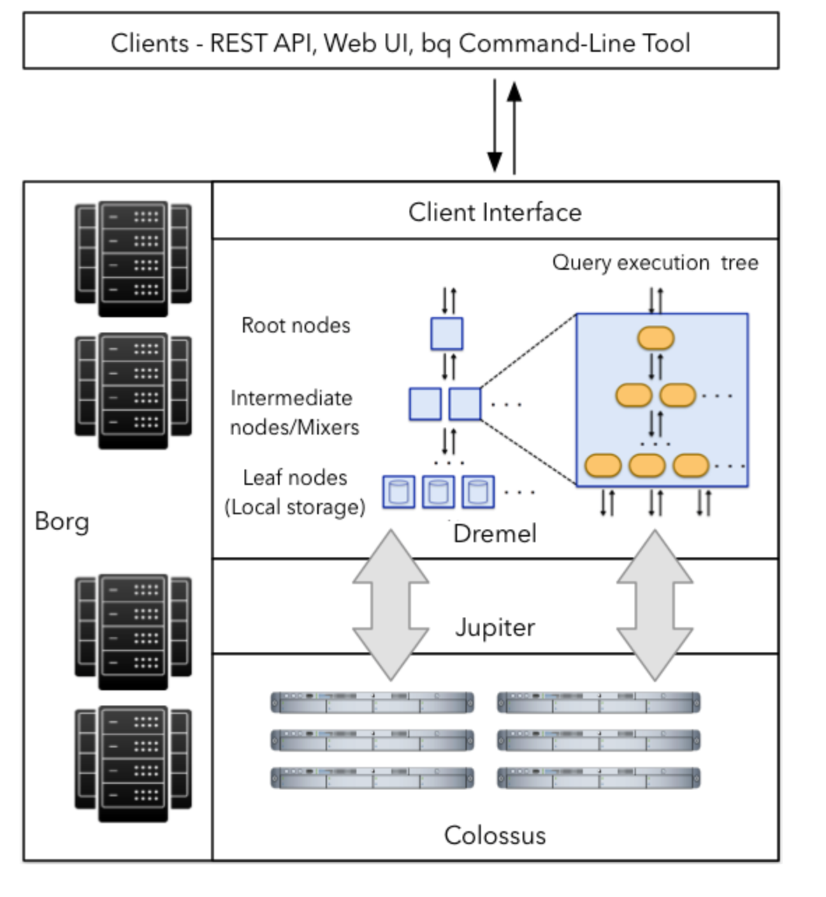
In the middle of this process, we are also dealing with spinning up APIs to access all of this on a per-project basis, and don’t forget that we are accessing the data from BigQuery. I’ve deliberately left out explaining absolutely anything about how BigQuery works, because that’s a topic big enough for another blog post, but if you are working with BigQuery, you also need to understand it as well. The TL;DR is that BigQuery is a group of technologies run on Google’s Colossus Storage which uses Dremel as its processing engine and Borg (pre K8s-K8s) to access and run distributed data operations to bring your data back for you.
So by the end of this, we have build a model of where we need to look for bottlenecks, and it looks like this:
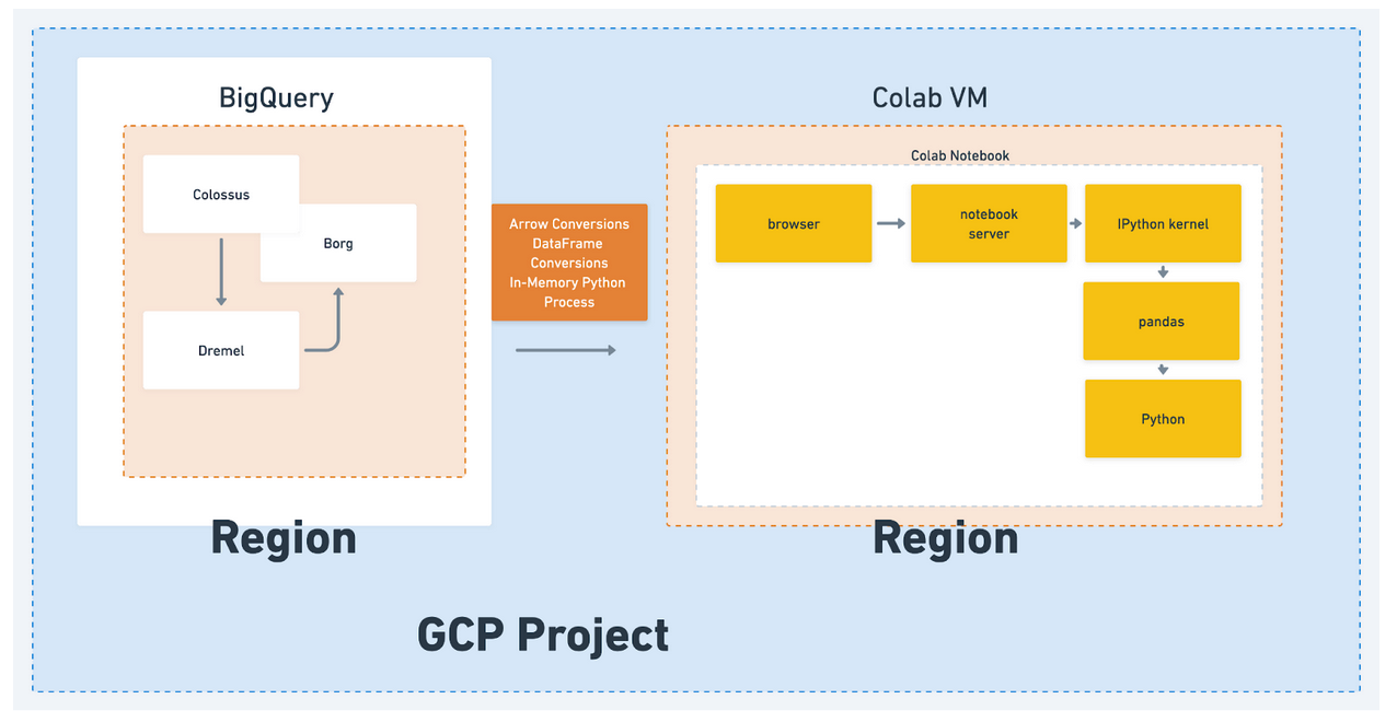
Because we also need to account for the region and availability zone, the logical project separation, and any other APIs connecting BigQuery and Colab. These are only the things I can think of off the top of my head and don’t include any meta-programming work, such as setting up configuration, security, and all the work that happens around the cloud.
Whereas before we just had our small Python interpreter and our local shell, now we are at least 5-6 layers away from potentially finding the memory issue and figuring out what to do with it, in an API that blocks us from doing any real programming and has us looking between the components.
The answer, in the cloud, is to just use a bigger instance, until you get to the point where your process fits in-memory, and gluing together BQ, Notebooks, queries, and so on until infinity, unable really to get to the heart of the matter.
I should note that upgrading to Colab Pro, which is opaque around how big the image actually ends up being, did not even solve this problem (it doubles, to 26 GB RAM.)
A larger problem than memory
All of this is deeply unsatisfying to me and ties into the holistic problem I have with modern software development.
Modern software is hard to develop locally, hard to build the internal logic for, and intrinsically hard to deploy, especially so in the case of machine learning. Just take a look at the MLOps paper, which I have nightmares about occasionally.
The problem has gotten so bad that you can usually no longer start from scratch and develop and test a single piece of software in a single, preferably local environment.
In order to re-create Viberary locally, I would have to somehow spin up BigQuery? Then also somehow recreate Colab, which, again, is proprietary, and test there.
Once in production, I will have to abstract everything away through networking and layers and layers of service accounts, with the vendor in the way and looking out for their own best interests instead of how we want to work as developers. The actual logic of our program becomes almost invisible, buried among services and APIs.
To be clear, the situation is not all bad. There is much that we gain when we go to the cloud. For example, in no previous universe would I be able to try out Stable Diffusion, spin up enormous Spark clusters, or even contemplate Viberary as a project. I wouldn’t be able to do end-to-end machine learning inference, build fun applications, or do most of the things that modern GitHub gives us.
And, also, we don’t need to go back to the mainframe or writing assembly. We just need to step back from the cloud insanity ledge a little bit. The pros that we get when we program in this way are outweighed by what we give up, and it is this heart of engineering that I find myself missing the most.