Welcome to the jungle, we got fun and frames
This is part of a series of posts on building Viberary, a semantic search/recommendation engine for vibes and what happens when you have unlimited time to chase rabbit holes in side projects.
I’m still in the early stages of this project and doing data analysis on the input data, a dump of 10GB from Goodreads in JSON. See the input data sample here.
Last time I left off, I was working with a BigQuery table I had created from the initial JSON file and trying to read into pandas via the BigQuery connector. That didn’t work well because of in-memory issues, but I didn’t have enough information about the BigQuery and Colab proprietary environments to dig too far into the performance bottleneck, which I was pretty sure was the BigQuery connector iterator class.
In order to move onto my next step, learning an embeddings model for both the books dataset and the query I end up generating, either via BERT or word2vec, I need to check out the data and then, format it for processing.
The easiest way to look at data at a glance in the data science space is still Pandas DataFrames, so I thought that if I took the complication of the cloud out of this, I could read this data into a local Pandas DataFrame to perform some summary stats on it.
None of this needs to be in pandas, actually, but that is the standard industry way to do data analysis these days, I know it fairly well, and it works pretty easy locally. The data file itself is 2 GB zipped, 9GB unzipped, which based on the Boykis rule of thumb, should be just small enough to work with locally.

Or so I thought. When I tried to use read_json in Pandas, the kernel took over 2 minutes just to read the data in. Actually, initially I wasn’t sure if it would even be able to read the entire file, and I’d need to read it in again and again during the exploration process, so this wasn’t an optimal way to go.
But to understand the performance constraints, I had to go pretty deep into the Pandas ecosystem.
Pandas building blocks
In order to understand Pandas, one must become one with the DataFrame Let’s take DataFrames apart into their components.
First, we have a Series. A series is like an ndarray, which are arrays that are specifically optimized for mathematical computing in the numpy ecosystem.
The other part of a Series is that they are labeled with the row header, so that you can access them by the label. In this way, they are also like Python dictionaries.
import numpy as np
s = pd.Series(np.random.randn(5), index=["item1", "item2", "item3", "item4", "item4"])
item1   -0.994375
item2   -0.663550
item3   -0.059189
item4   -1.001517
item4    0.010971
dtype: float64

t = pd.Series(np.random.randn(5), index=["item1", "item2", "item3", "item4", "item4"])
item1   -1.295399
item2    0.678834
item3   -0.095558
item4    1.308766
item4   -1.043527
dtype: float64
Combining a number of these dictionary-like Series structures together gives you a DataFrame.
df3 = pd.DataFrame({"one":s,"two":t},index=["item1", "item2", "item3", "item4", "item4"])
 	one 	two
item1 	-1.457448 	-0.614105
item2 	0.622242 	0.641537
item3 	1.433366 	-0.684267
item4 	0.695813 	-1.294600
item4 	1.549621 	0.682719
So a way to think of a DataFrame is a dictionary of dictionary-like objects.
Under the hood, these dictionary-like objects are actually collections of arrays. The array piece is crucial to understanding the performance limitations of pandas.
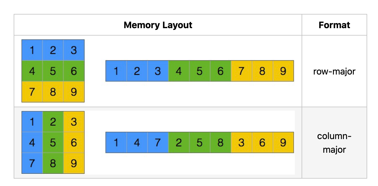
Array data structures in computer science in general and in Python numerical computing specifically are fixed-width, which makes it easy to retrieve items at specific indices.
But what this means at write time is that, when we create them, we pre-allocate specific amounts of memory, sometimes much more than we need, so that we can read them into memory.
An instance of class ndarray consists of a contiguous one-dimensional segment of computer memory (owned by the array, or by some other object), combined with an indexing scheme that maps N integers into the location of an item in the block. The ranges in which the indices can vary is specified by the shape of the array. How many bytes each item takes and how the bytes are interpreted is defined by the data-type object associated with the array.
In numpy, we specify this explicitly. When we create DataFrames, Pandas abstracts away this specification for us. Often what it means is that DataFrames are very memory-efficient on read, but not on write and create enormous RAM performance hits. See this excellent explainer which this image comes from for more.
Profiling Pandas
How memory-inefficient are DataFrames? No one has been able to give a definite answer since benchmarks are hard. For example, Peter found (https://colab.research.google.com/drive/1TWa9L5NQE-cBYOpFvzwSu7Rjoy6QtFWw) that memory required for a 100MB CSV file peak memory use for loading and writing the file was 4.4-7.7x the file size.
As I sit down to write this, the third-most popular pandas question on StackOverflow covers how to use pandas for large datasets. This is in tension with the fact that a pandas DataFrame is an in memory container. You can’t have a DataFrame larger than your machine’s RAM. In practice, your available RAM should be several times the size of your dataset, as you or pandas will have to make intermediate copies as part of the analysis.
Perhaps the single biggest memory management problem with pandas is the requirement that data must be loaded completely into RAM to be processed. pandas’s internal BlockManager is far too complicated to be usable in any practical memory-mapping setting, so you are performing an unavoidable conversion-and-copy anytime you create a pandas.DataFrame.
It can be insanely hard, because of this and because of the way pandas internals are laid out, to benchmark.
In our case, in addition to internals, these benchmarks will need to account for:
- Hardware
- The version of Pandas we’re running (and Jupyter and any additional file processing utilities outside of Python’s standard library)
- The file type we’re ingesting
- The size of the file
- The type of data in the file and number of columns (i.e. numerical data is more efficient than textual data and different kinds of numerical data take up less space than others:
For example, int64 uses 4× as much memory as int16, and 8× as much as int8. By default when Pandas loads a CSV, it guesses at the dtypes. If it decides a column volumes are all integers, by default it assigns that column int64 as the dtype. As a result, if you know that the numbers in a particular column will never be higher than 32767, you can use an int16 and reduce the memory usage of that column by 75%.
All of this makes for a hard task.
But we can do some eyeballing. I started by sampling the json file and seeing what the memory footprint of reading a single line in would be using memray, a Python memory profiling tool that now has notebook support:
df = json.read_json("/Users/vicki/viberary/viberary/jsonparquet/src/main/resources/goodreads_sample.json")

# total memory allocated for DF (h/t to [Peter for his beautiful notebook here](https://colab.research.google.com/drive/1TWa9L5NQE-cBYOpFvzwSu7Rjoy6QtFWw))
# taking the latest-generated file in the memray-results output by time and parse out performance metadata
latest_file = max(Path("memray-results/").glob("**/*.html"), key=os.path.getmtime)
soup = BeautifulSoup(latest_file.read_text())
stats = soup.find("div", {"id" : "statsModal"}).find("div", {"class" : "modal-body"})
print(stats.text)
        Command line: /usr/local/lib/python3.9/site-packages/ipykernel_launcher.py -f
/Users/vicki/Library/Jupyter/runtime/kernel-87e391e0-0452-4dc9-bbd9-48ccec32f39e.json
          Start time: 2023-01-11 13:15:56.652000
          End time: 2023-01-11 13:15:56.705000
          Total number of allocations: 974
          Total number of frames seen: 78
          Peak memory usage: 19.3 kB
          Python allocator: pymalloc
This tells us that, when running read_json, pymalloc allocates 19.3 kb to read, process, and parse a single JSON row. Here’s everything
it needs to do:
- First, it does a bunch of preprocessing to check the data and directory
- Then, it combines everything from the file into a single JSON object
- Then, it reads the entire JSON object as a string into pandas
- The amount of parsing that happens is not insignificant
Not only is there CPU processing happening, there are also I/O operations happening concurrently, and memory in RAM is being allocated contiguously to store the DataFrame that’s being built in-memory.
So, given all of this,if one JSON array is 19 kb, how much memory can we expect my file, which is approximately 2.3 mil rows (or JSON objects) to take?
19.3 kB * 2.3 million = 43.7 GB
This is assuming all of this computational cost scales linearly and we don’t have O(n log n) or worse performance as we add more in-memory objects and indices and other overhead to keep track of them.
No wonder my original Colab notebook wasn’t able to handle it; even at the Pro level, Colab “only” allocates 26 GB RAM.
This seems insane given that Apollo Guidance Computer had 4KB of RAM.
I’m not going to the moon here, I’m just working on shitposting my way through a semantic search embeddings project.
Improving performance through iteration on input data formats
There are a number of different ways we can improve read-through performance here: reading less rows, selecting the columns we’d like ahead of time so that we’re not processing text-heavy nested JSON, optimizing data formats, and trying different approaches outside of Pandas, such as Polars and DuckDB, which are two prominent alternatives that have recently started their rise in the data space.
Since I’d already spent so much time thinking about Pandas, my initial approach was to see if I could tune my raw JSON input.
There are, without question, [data formats that perform better in Pandas than others.](https://pandas.pydata.org/docs/user_guide/enhancingperf.html) These are:
- Parquet. This is a format that’s used all over big data land, originally created for use in the Hadoop ecosystem but now frequently used in conjunction with Spark/DeltaLake. It uses a self-described schema and is optimized for storage and querying in columnar format. However, in order to work with it in-memory for large files, you need to stream Parquet files.
It’s supported by a number of different tools including Spark, Hive, Impala, and BigQuery, which I’ll be working with later
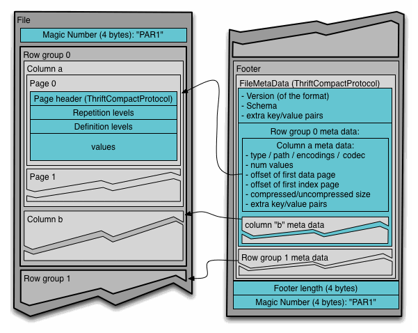
- Arrow is a also a columnar format that’s meant less for storage and more for in-memory analytics. It’s intended to be compatible with Parquet; i.e. you can read an Parquet file using Arrow into memory, and in fact the
read_parquetmethod in Pandas defaults to the Python implementation of arrow, pyarrow. - Feather is yet another columnar disk storage format, tied closely to Arrow to also allow for fast reads/writes, but I haven’t seen this one developed as much as the others.
Something you’ll notice that’s common between these performant file formats is they all operate on columns versus rows, and it’s this that, among other considerations make it easier to read into Pandas because as you’ll remember from earlier in the post, DataFrame fundamental building blocks are column vectors or arrays that we add together with an index to create our row-based DataFrame table.
But ultimately what makes these easier to work with, particularly with JSON, is a pre-specified schema so that pandas doesn’t have to work hard figuring out datatypes.
Given all these choices, I tried several different approaches:
- Loading the raw JSON file
          Command line: /usr/local/lib/python3.9/site-packages/ipykernel_launcher.py -f
/Users/vicki/Library/Jupyter/runtime/kernel-87e391e0-0452-4dc9-bbd9-48ccec32f39e.json
          Start time: 2023-01-12 16:13:05.618000
          End time: 2023-01-12 16:13:34.124000
          Total number of allocations: 30
          Total number of frames seen: 47
          Peak memory usage: 55.2 GB
          Python allocator: pymalloc
   ~ 29 secs
- Loading into a PyArrow table and then to a DataFrame
Command line: /usr/local/lib/python3.9/site-packages/ipykernel_launcher.py -f
/Users/vicki/Library/Jupyter/runtime/kernel-87e391e0-0452-4dc9-bbd9-48ccec32f39e.json
          Start time: 2023-01-12 16:35:17.344000
          End time: 2023-01-12 16:37:22.167000
          Total number of allocations: 42194315
          Total number of frames seen: 76
          Peak memory usage: 45.0 GB
          Python allocator: pymalloc
- Creating a Parquet file and loading that directly into a DataFrame
Command line: /usr/local/lib/python3.9/site-packages/ipykernel_launcher.py -f
/Users/vicki/Library/Jupyter/runtime/kernel-87e391e0-0452-4dc9-bbd9-48ccec32f39e.json
          Start time: 2023-01-12 16:30:36.757000
          End time: 2023-01-12 16:32:20.668000
          Total number of allocations: 12185306
          Total number of frames seen: 115
          Peak memory usage: 45.3 GB
          Python allocator: pymalloc
With memray once you set it up correctly, you also get these really nice visuals:
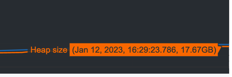
The last two take longer but are more efficient memory-wise, because we’re now specifying a schema at read time. Using a Parquet file directly is your best bet, in this very specific case, taking up 45.3 GB of ram in memory and slightly less than 2 min.
The interesting part of creating a Parquet file is that, in the year of our lord 2023, Parquet files are everywhere. They’re inputs and outputs for Spark and DeltaLake, DuckDB supports them,and there are hundreds of millions of files sitting across various data lakes and lakehouses and lake mansions in S3 quietly in parquet format, waiting to be modeled.
So, why, in the year of our lord 2023, is SO hard to find a standalone utility to create Parquet files?

You can create Parquet files in Spark and in DuckDB and in clickhouse, but you have to download those computational systems first and read the data into those systems first. Why can’t I just download some cli utility that does this?
It seemed strange that there was no stand-alone tool for this. Parquet-tools also partially does this, but you have to manually create a an Avro schema that will be bound to the parquet file.
So, of course, I started working on a small utility to do this. But what I found was that the tooling for Parquet in Java, the original language of data lakes and Hadoop file systems and where Parquet sprung out of, was surprisingly out of date.
It’s also very closely tied (understandably) to the Hadoop filesystem, where Parquet began its life.
By the end of hunting down Avro/Parquet conversion loopholes, out-of-date Kite dependencies and trying to read .avsc files, what I realized I was spending more time writing the utility than benchmarking and moving onto the modeling, and I cheated slightly by reading the JSON file into a local instance of Spark and writing out to Parquet. An issue here is that you still cannot specify a default schema file unless you do a column-by-column projection using withColumn in Spark, I’m guessing because Catalyst optimizes it, so I had to do even further work in Pandas to get the numerical columns into the shape I wanted.
Arrow and Parquet are very very close with Parquet being slightly slower, which makes sense since it’s optimized for storage and not in memory-analytics, but the benefit of using Parquet is that I can use the file format everywhere else, including BigQuery, so that’s what I’m going to go with.
Except, however, when I read the data in, I ran into another problem: datatypes.
You may recall that the original JSON file looks like this:
"isbn": "0413675106",
  "text_reviews_count": "2",
  "series": [
    "1070125"
  ],
  "country_code": "US",
  "language_code": "",
  "popular_shelves": [
    {
      "count": "2979",
      "name": "to-read"
Can you spot the issue? Yes! the numerical fields are coded as text fields in the original file. So, even if you create a Parquet file, unless you are hand-writing the Avro schema, which I was not able to do in either my stand-alone utility or in Spark, it will say that all your fields are text, and you will have to do a conversion.
# convert to numerical types for working
df_parquet['average_rating'] = pd.to_numeric(df_parquet['average_rating'],errors="coerce")
df_parquet['num_pages'] = pd.to_numeric(df_parquet['num_pages'],errors="coerce")
df_parquet['publication_day'] = pd.to_numeric(df_parquet['publication_day'],errors="coerce")
df_parquet['publication_month'] = pd.to_numeric(df_parquet['publication_month'],errors="coerce")
df_parquet['publication_year'] = pd.to_numeric(df_parquet['publication_year'],errors="coerce")
df_parquet['ratings_count'] = pd.to_numeric(df_parquet['ratings_count'],errors="coerce")
df_parquet['text_reviews_count'] = pd.to_numeric(df_parquet['text_reviews_count
This is an enormous pain, and it saves some space in the in-memory DataFrame object but the resulting object is enormous ,which ends up being over 6GB in-memory as-is. If you recall, our original file was 9GB.
It’s clear which the text fields are here:
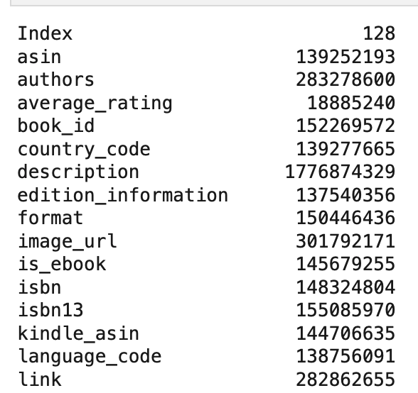
I could kind of work with this, but it was really hard, and it took me a long time to get here.
Trying a few different libraries: Polars
The sexy new kid on the block is Polars. Everyone is talking about it and everyone is doing it. I tried two different times, once when I was reading data from BigQuery and again when I was looking to parse my JSON. Both times, I got inexplicable errors I spent 10-15 minutes digging into before I stopped. The second time, while working with Polars locally, my Jupyter kernel immediately OOMed, likely related to the fact that Polars does not yet have a good way to deal with JSON parsing.
Reading from parquet directly also immediately resulted in a dead kernel and kernel panic.
import polars as pl

%%memray_flamegraph
df = pl.read_parquet("/Users/vicki/viberary/viberary/jsonparquet/src/main/resources/goodreads.parquet")
Since I’d rather troubleshoot data and model issues at this point, I’m leaving polars to try for another time, but it’s still top of mind for me.
DuckDB
You may guess where this is all headed by now, and, because the DuckDB fan club is extremely vocal and loud, I thought I’d see what the fuss is about. DuckDB is everyone’s favorite venture-capital backed SQLLite-like database that is tuned specifically to work for on analytical workloads, aka reads in SQL from a database.
You can find all the reasons for using it everywhere online, it’s taken the analytics community by storm. There are a number of reasons why, and after going through the wilderness of my Pandas/Parquet journey, I can see why: it makes all the stuff I was having to thinking about easy.
In my case, it was important for me to go through this Journey so I could better understand all the internal components.
DuckDB is a nice tool, but it is not a miracle worker. Although it read in my parquet file directory fairly quickly , it still couldn’t infer types correctly from the JSON file, which makes sense, since, as this exercise has proved, JSON is a cursed format:
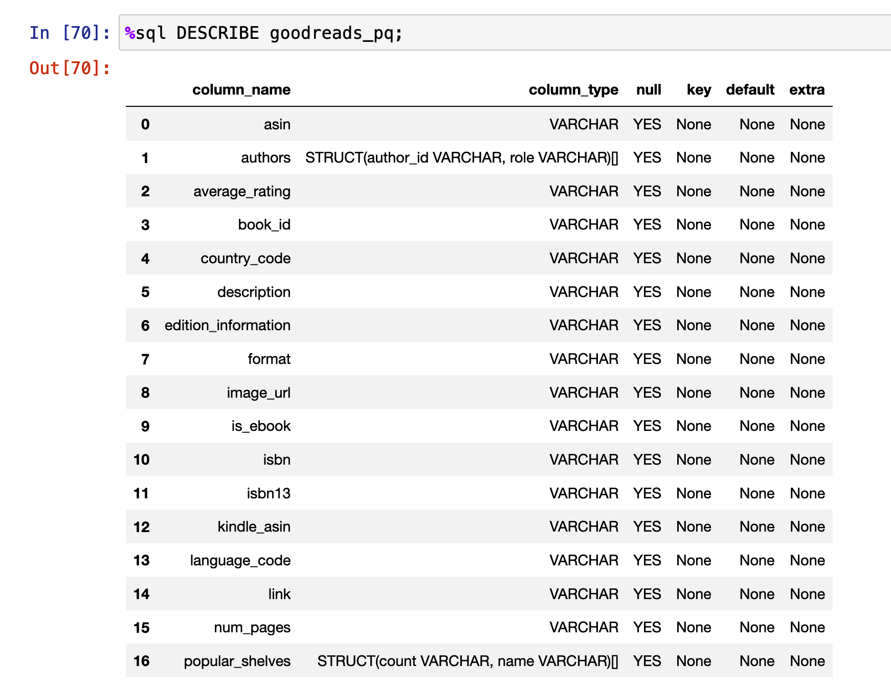
Here are extra attempts I did to get it to work, and even in this case, you can see that it didn’t render null strings correctly, which was also the case with Pandas:

So I eventually had to cast at the column level in my queries:
%sql my_df << SELECT try_cast(num_pages as INTEGER), count(*) AS total_books \
FROM goodreads_pq \
GROUP BY num_pages \
ORDER BY count(*) desc;
The difference between DuckDB and pandas is that it performs these casts and aggregations fairly easily.
And, critically for me, it easily exports in-memory objects to Pandas so that you can use Pandas for what the Good Lord meant pandas to be used for, which was not introspecting memory performance, but plotting small pieces of data and understanding them in Jupyter notebooks
You can see the notebook I created with the JSON file here.
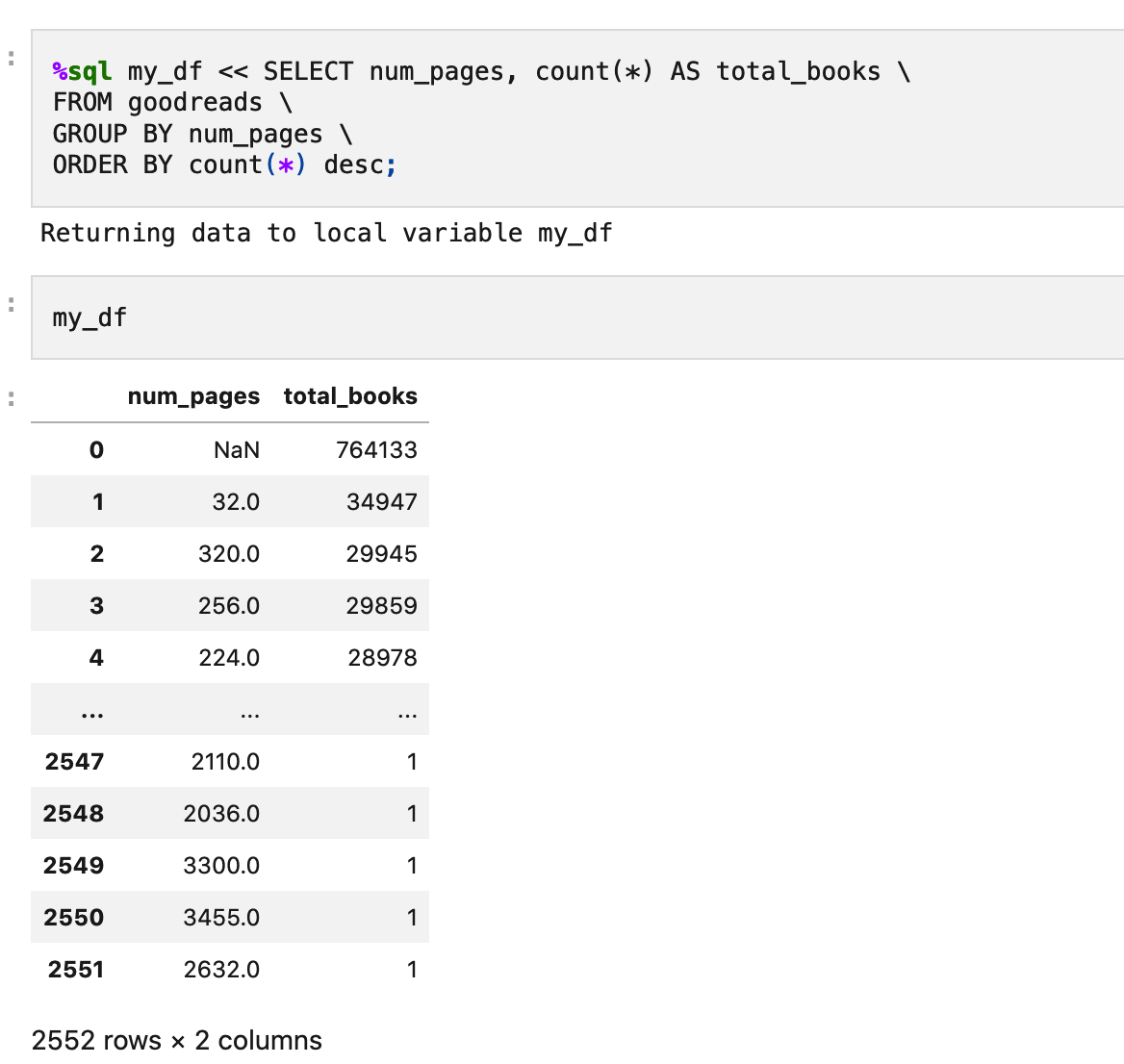
It’s not immediately clear to me that DuckDB is better for my specific use case and it still had trouble with both JSON and Parquet, but it works easy enough, easier than Pandas out of the box, enough for me to continue on to data analysis, for now.
TL;DR:
- Do not use data formatted as JSON, you are going to have a bad time in any tool you use. Especially if the data is hard-coded as strings. If it’s not your data, sorry you’re dealing with it, and if it’s yours, sorry you did this to yourself.
- Schemas and schema-defined formats exist for a reason, try to use them as much as possible, particularly parquet if you can, although generating and evolving parquet files is hard.
- Pandas is very, very bad at anything above, say, 5 GB and at this point you should likely switch to another tool that performs your aggregations
- Pandas memory profiling is basically a black box and even smart people have given up on this. Try a different tool if you find yourself doing deep copies on DataFrame memory.
Now, my own RAM is entirely full of RAM and performance facts and I’m ready to leave it all behind so I can move onto the data analysis and learn some embeddings!
#data #python #data science #big data #data formats