Retro on Viberary

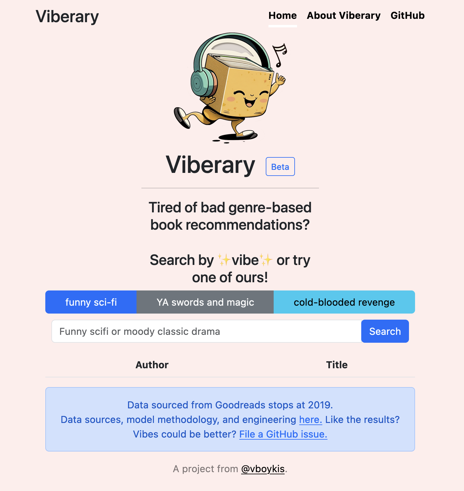
Viberary is a side project that I worked on in 2023, which does semantic search for books by vibe. It was hosted at [viberary.pizza.]
I’m shutting down the running app and putting the codebase in maintenance mode because:
- A lot of what I want to continue to do there (i.e. changing embedding models, modifying training data) involves building out more complex infra: a model store, a feature store, data management, evaluation infra, and all of that’s going to take longer than I have
- There’s a lot of maintenance that needs to happen for a running app (Python dependencies, etc. ) I.e. all code is technical debt.
- Cost! I don’t want to maintain an app that is currently losing $100+ a month to maintenance costs unless I’m also planning to make money from it. I’m not planning to, but I have learned a LOT from this project and I have loved building and sharing it.
- I have a new project idea I’d like to work on, so I need to make space for it.
There were SO many, SO many things I learned from this project. Most of them are outlined in the post below, so read on. But, if you want a list of high-level bullets:
- The project HAS to be something you’re interested in. You will not work on it otherwise. I love books and I want to be recommended books, and I had a keen understanding of this problem space before I started.
- Start as simple as you can, but no simpler. You should be able to test anything you deploy locally without external dependencies. You need to be able to go fast at the beginning, otherwise you’ll lose interest.
- At the same time, you will not know what’s simple unless you try something, anything.
- Simple means most of the code you write should be your library logic, not glue code between cloud components.
- Docker on new Mac M1+ architectures that have to be ported to Linux is really annoying but fixable.
- Knowing nginx well can save you a ton of time
- Sometimes you don’t need large language models, BERT works just fine
- Evaluating the results of unsupervised ranking and retrieval is really hard and no one has solved this problem yet
- Digital Ocean has an amazing product suite that just works for small and medium-size projects
- The satisfaction of shipping products that you’ve build is unparalleled
For much, much more, read on!
August 5, 2023
TL;DR: Viberary is a side project that I created to find books by vibe. I built it to satisfy an itch to do ML side projects and navigate the current boundary between search and recommendations. It’s a production-grade complement to my recent deep dive into embeddings.
This project is a lot of fun, but conclusively proves to me what I’ve known all along about myself: reaching MLE (machine learning enlightenment) is the cyclical process of working through modeling, engineering,and UI concerns, and connecting everything together - the system in production is the reward. And, like any production-grade system, machine learning is not magic. Even if the data outputs are not deterministic, it takes thoughtful engineering and design choices to build any system like this, something that I think gets overlooked these days in the ML community.
I hope with this write-up to not only remind myself of what I did, but outline what it takes to build a production Transformer-based machine learning application, even a small one with a pre-trained model, and hope it serves as a resource and reference point.
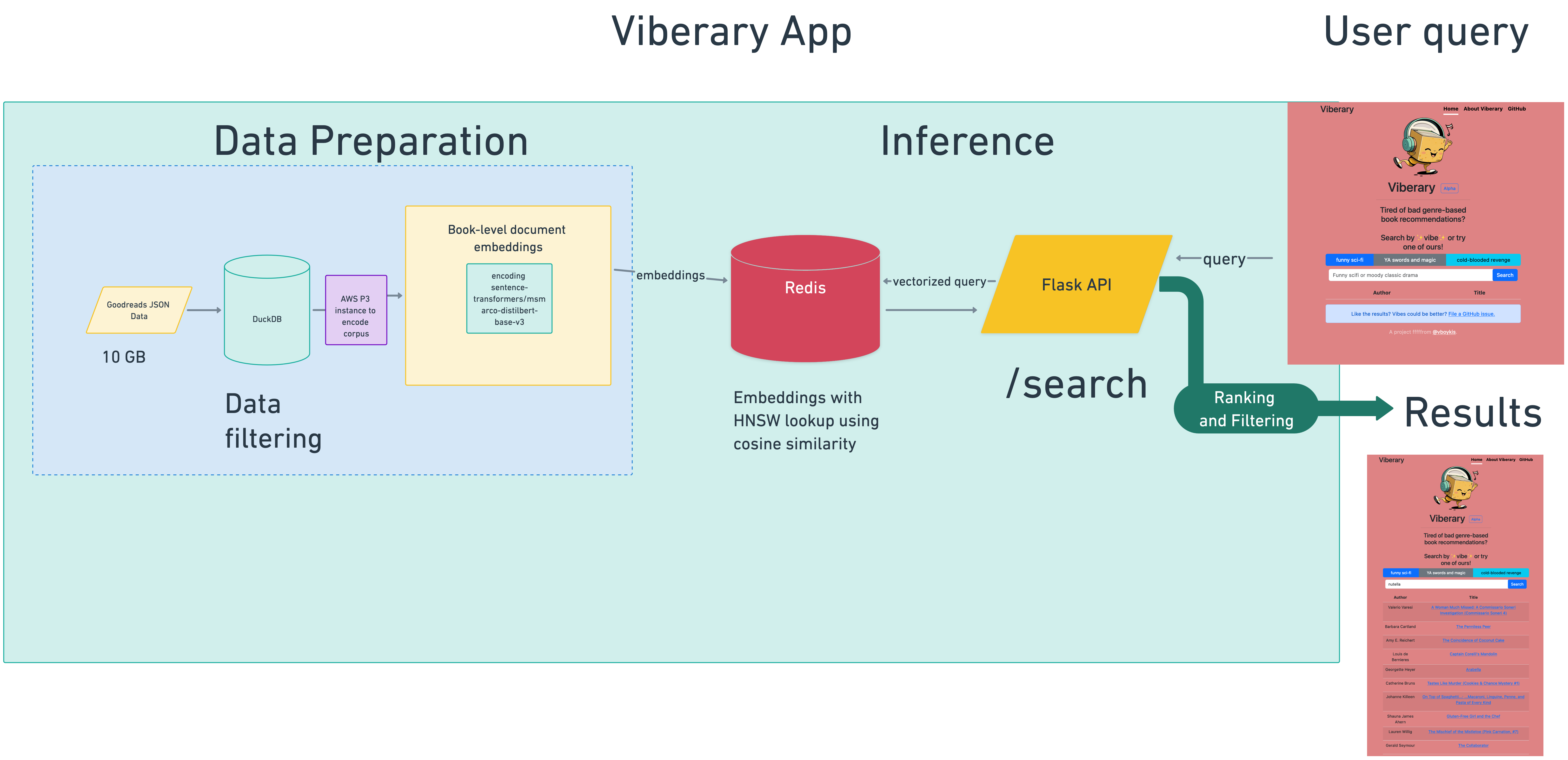
Viberary’s machine learning architecture is a two-tower semantic retrieval model that encodes the user search query and the Goodreads book corpus using the Sentence Transformers pretrained asymmetric MSMarco Model.
The training data is generated locally by proessing JSON in DuckDB and the model is converted to ONNX for performant inference, with corpus embeddings learned on AWS P3 instances against the same model and stored in Redis. Retrieval happens using the Redis Search set with the HNSW algorithm to search on cosine similarity. Results are served through a Flask API running four Gunicorn workers and served to a Bootstrap front-end. using Flask’s ability to statically reder Jinja templates. There is no Javascript dependencies internal to the project.
It’s served from two Digital Ocean droplets behind a Digital Ocean load balancer and Nginx, as a Dockerized application with networking spun up through Docker compose between the web server and Redis Docker image, with data persisted to external volumes in DigitalOcean, with [Digital Ocean] serving as the domain registrar and load balancer router.
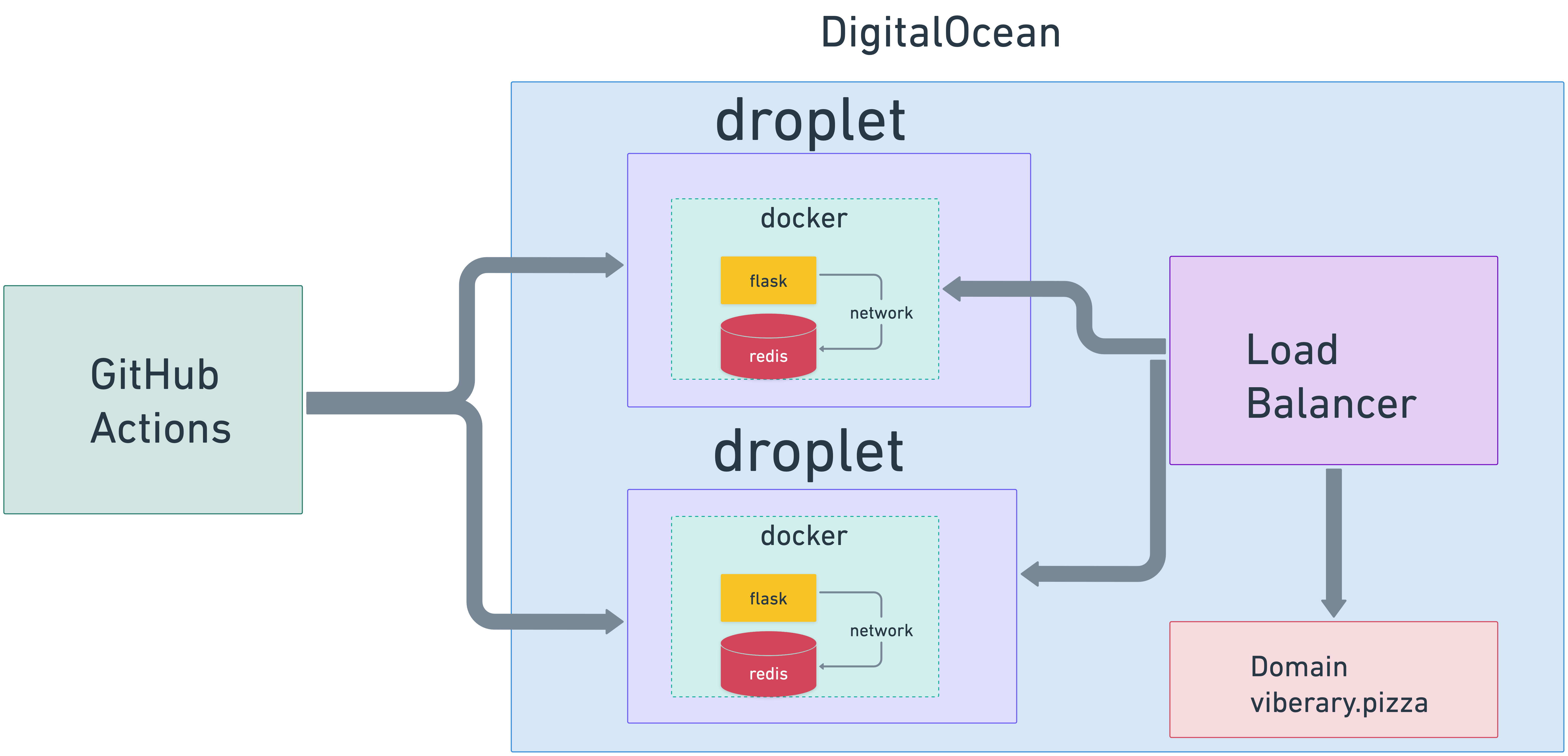
The deployable code artifact is generated through GitHub actions on the main branch of the repo and then I manually refresh the docker image on the droplets through a set of Makefile commands. This all works fairly well at this scale for now.
What is semantic search?
Viberary is a semantic search engine for books. It finds books based on ✨vibe✨. This is in contrast to traditional search engines, which work by performing lexical keyword matching on terms like exact keyword matches by genre, author, and title - as an example, if you type in “Nutella” into the search engine, it will try to find all documents that specifically have the word “Nutella” in the document.
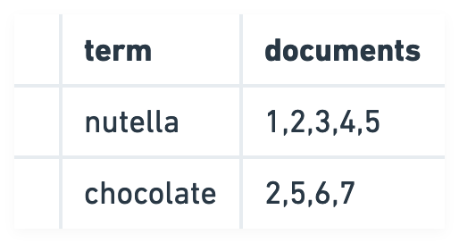
Traditional search engines, including Elasticsearch/OpenSearch do this lookup efficiently by building an inverted
index, a data structure that creates a
key/value pair where the key is the term and the value is a collection of all the documents that match the term and performing retrieval from the inverted index. Retrieval performance from an inverted index can vary depending on how it’s implemented, but it is O(1) in the best case, making it an efficient data structure.
A commonc classic retrieval method from an inverted index is BM25, which is based on TF-IDF and calculates a relevance score for each element in the inverted index. The retrieval mechanism first selects all the documents with the keyword from the index, the calculates a relevance score, then ranks the documents based on the relevance score.
Semantic search, in contrast, looks for near-meanings based on, as “AI-Powered Search” calls it, “things, not strings.” In other words,
“Wouldn’t it be nice if you could search for a term like “dog” and pull back documents that contain terms like “poodle, terrier, and beagle,” even if those document happen to not use the word “dog?”
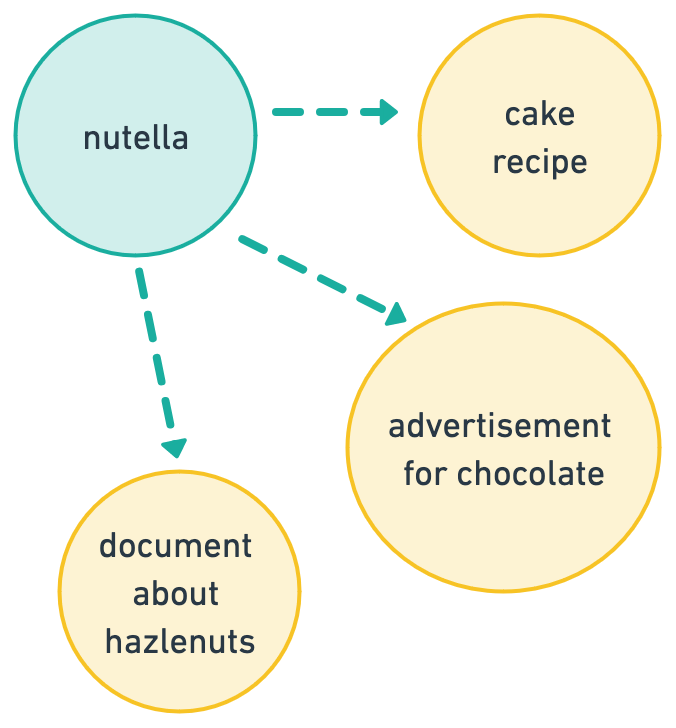
Semantic search is a vibe. A vibe can be hard to define, but generally it’s more of a feeling of association than something concrete: a mood, a color, or a phrase. Viberary will not give you exact matches for “Nutella”, but if you type in “chocolately hazlenut goodness”, the expectation is that you’d get back Nutella, and probably also “cake” and “Ferrerro Rocher”.
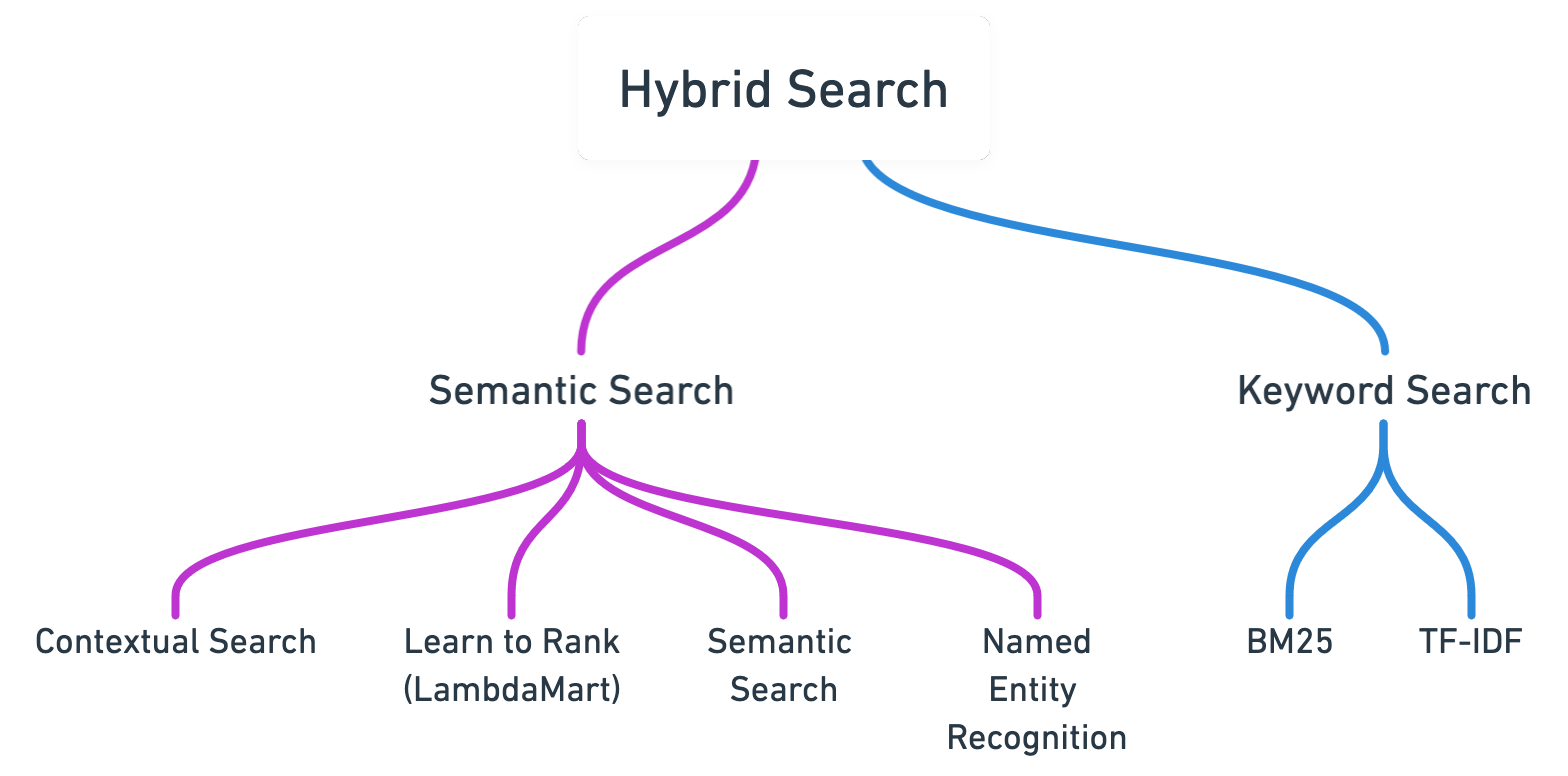
Typically today, search engines will implement a number of both keyword-based and semantic approaches in a solution known as hybrid search. Semantic search includes methods like learning to rank, blending several retrieval models, query expansion which looks to enhance search results by adding synonyms to the original query, contextual search based on the user’s history and location, and vector similarity search, which looks to use NLP to help project the user’s query in a vector space.
The problem of semantic search is one researchers and companies have been grappling with for decades in the field known as information retrieval, which started with roots in library science. The paper introducing Google in 1998 even discusses the problems with keyword-only search,
"People are likely to surf the web using its link graph, often starting with high quality human maintained indices such as Yahoo! or with search engines. Human maintained lists cover popular topics effectively but are subjective, expensive to build and maintain, slow to improve, and cannot cover all esoteric topics. Automated search engines that rely on keyword matching usually return too many low quality matches."The tension of the ability to make search engines work effectively in the space between [query understanding](https://queryunderstanding.com/) through human enrichment and getting machines to better understand user intent has always been present.
Netflix was one of the first companies that started doing vibe-based content exploration when it came up with a list of over 36,000 genres like “Gentle British Reality TV” and “WitchCraft and the Dark Arts” in the 2010s. They used large teams of people to watch movies and tag them with metadata. The process was so detailed that taggers received a 36-page document that “taught them how to rate movies on their sexually suggestive content, goriness, romance levels, and even narrative elements like plot conclusiveness.”
These labels were then incorporated into Netflix’s recommendation architectures as features for training data.
It can be easier to incorporate these kinds of features into recommendations than search because the process of recommendation is the process of implicitly learning user preferences through data about the user and offering them suggestions of content or items to purchase based on their past history, as well as the history of users across the site, or based on the properties of the content itself. As such, recommender interfaces often include lists of suggestions like "you might like.." or "recommended for you", or "because you interacted with X.."
Search, on the other hand, is an activity where the user expects their query to match results exactly, so users have specific expectations of modern search interfaces:
- They are extremely responsive and low-latency
- Results are accurate and we get what we need in the first page
- We use text boxes the same way we have been conditioned to use Google Search over the past 30 years in the SERP (search engine results page)
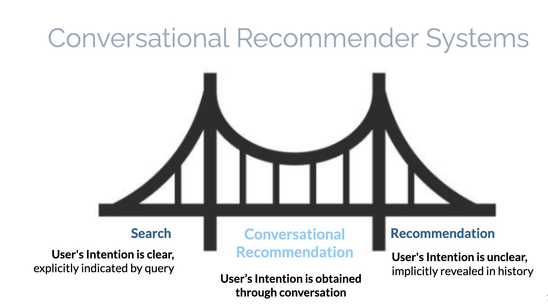
As a result, in some ways, there is a tension between what makes traditional search interface and semantic search successful respectively, because semantic search is in that gray area between search and recommendations and traditional search expects exact results for exact queries. These are important aspects to keep in mind when designing conversational or semantic search interfaces. For more on this, check out this recent article on Neeva.
Many search engines today, Google included, use a blend of traditional keyword search and semantic search to offer both direct results and related content, and with the explosion of generative AI and chat-based search and recommendation interfaces, this division is becoming even blurrier.
Why semantically search books?
I love reading, particularly fiction. I am always reading something. Check out my past reviews 2021, 2020, 2019, and you get the idea. As a reader, I am always looking for something good to read. Often, I’ll get recommendations by browsing sites like LitHub, but sometimes I’m in the mood for a particular genre, or, more specifically a feeling that a book can capture. For example, after finishing “The Overstory” by Richard Powers, I was in the mood for more sprawling multi-generational epics on arcane topics (I know so much about trees now!)
But you can’t find curated, quality collections of recommendations like this unless a human who reads a lot puts a list like this together. One of my favorite formats of book recommendations is Biblioracle, where readers send John Warner, an extremely well-read novelist, a list of the last five books they’ve read and he recommends their next read based on their reading preferences.
Given the recent rise in interest of semantic search and vector databases, as well as the paper I just finished on embeddings, I thought it would interesting if I could create a book search engine that gets at least somewhat close to what book nerd recommending humans can provide out of the box.
I started out by formulating the machine learning task as a recommendation problem: given that you know something about either a user or the item, can you generate a list of similar items that other users like the user has liked? We can either do this through collaborative filtering, which looks at previous user-item interactions, or content filtering, which looks purely at metadata of the items and returns similar items. Given that I have no desire to get deep into user data collection, with the exception of search queries and search query result lists, which I currently do log to see if I can fine-tune the model or offer suggestions at query time, collaborative filtering was off the table from the start.
Content-based filtering, i.e. looking at a book’s metadata rather than particular actions around a piece of content, would work well here for books. However, for content-based filtering, we also need information about the user’s preferences, which, again, I’m not storing.
What I realized is that the user would have to provide the query context to seed the recommendations, and that we don’t know anything about the user. At this point, based on this heuristic, it starts to become a search problem.
An additional consideration was that recommendation surfaces are also traditionally rows of cards or lists that are loaded when the user is logged in, something that I also don’t have and don’t want to implement from the front-end perspective. I’d like the user to be able to enter their own search query.
This idea eventually evolved into the thinking that, given my project constraints and preferences, what I had was really a semantic search problem aimed specifically at a non-personalized way of surfacing books.
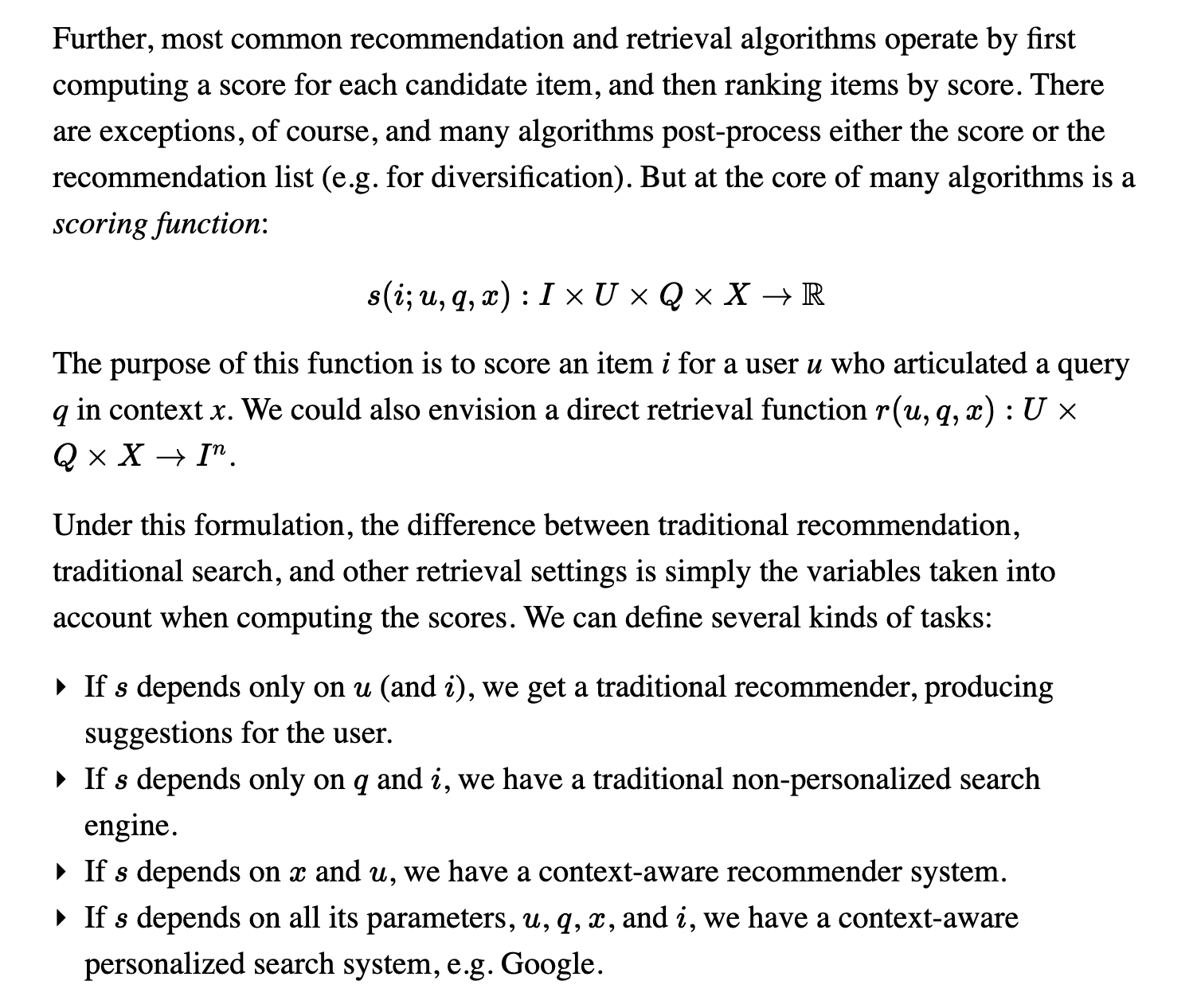
After a literature search,, what I found was a great paper that formulates the exact problem I wanted to solve, only in an ecommerce setting.
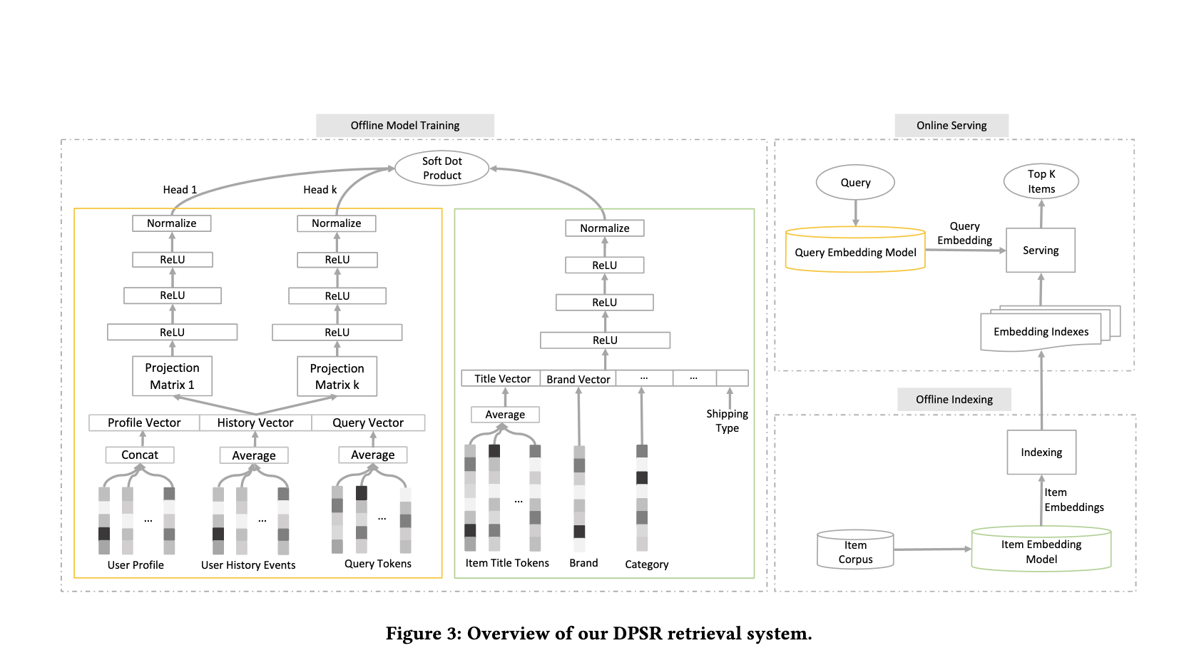
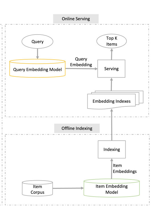
Their problem was more complicated in that, in addition to semantic search they also had to personalize it, and they also had to learn a model from scratch based on the data that they had, but the architecture was one that I could follow in my project, and the simplified online serving half was what I would be implementing.
Architecting Semantic Search
There are several stages to building semantic search that are related to some of the stages in a traditional four-stage recommender system:
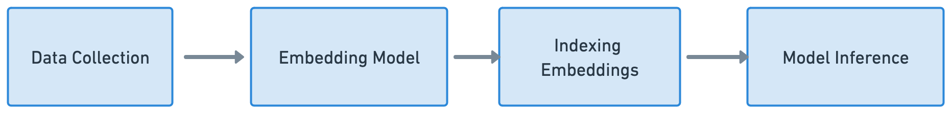
- Data Collection
- Modeling and generating embeddings
- Indexing the embeddings
- Model Inference, inclduing filtering
and a fifth stage that’s often not included in search/recsys architectures but that’s just as important, Search/Conversational UX design.
Most search and recommendation architectures share a foundational set of commonalities that we’ve been developing for years. It’s interesting to note that Tapestry, one of the first industrial recommender systems created in the 1990s to collaboratively filter emails, has an extremely similar structure to any search and recommendation system today, including components for indexing and filtering.
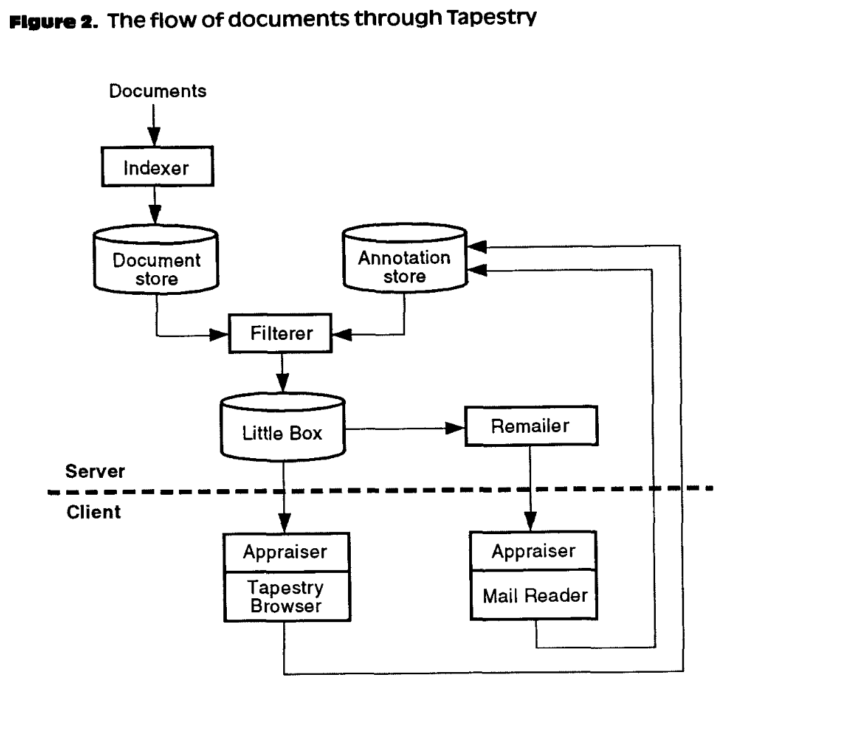
We start by collecting and processing a large set of documents. Our goal in information retrieval is to find the documents that are relevant to us, for any given definition of relevant. We update these collections of documents to be searchable at scale via an indexing function. We select a candidate set of relevant documents through either heuristics or machine learning. In our case, we do it by finding compressed numerical representations of text that are similar to the ones that we type into the query box. We generate these representations using an embedding space that’s created with deep learning models in the transformer family.
Then, once we find a candidate list of ~50 items that are potentially relevant to the query, we filter them and finally rank them, presenting them to the user through a front-end.
There are a number of related concerns that are not at all in this list but which make up the heart of machine learning projects: iteration on clean data, evaluation metrics both for online and offline testing, monitoring model performance in production over time, keeping track of model artifacts in model stores, exploratory data analysis, creating business logic for filtering rules, user testing, and much, much more. In the interest of time, I decided to forgo some of these steps as long as they made sense for the project.
Project Architecture Decisions
Given this architecture and my time constraints, I constrained myself in several ways on this project. First, I wanted to a project that was well-scoped and had a UI component so that I was incentivized to ship it, because the worst ML project is the one that remains unshipped. As Mitch writes, you have an incentive to move forward if you have something tangible to show to yourself and others.
I've learned that when I break down my large tasks in chunks that result in seeing tangible forward progress, I tend to finish my work and retain my excitement throughout the project. People are all motivated and driven in different ways, so this may not work for you, but as a broad generalization I've not found an engineer who doesn't get excited by a good demo. And the goal is to always give yourself a good demo.
Second, I wanted to explore new technologies while also being careful of not wasting my innovation tokens. In other words, I wanted to build something normcore, i.e. using the right tool for the right job, and not going overboard.. I wasn’t going to start with LLMs or Kubernetes or Flink or MLOps. I was going to start by writing simple Python classes and adding where I needed to as pain points became evident.
The third factor was to try to ignore the hype blast of the current ML ecsystem, which comes out with a new model and a new product and a new wrapper for the model for the product every day. It wasn’t easy. It is extremely hard to ignore the noise and just build, particularly given all the discourse around LLMs and now in society at large.
Finally, I wanted to build everything as a traditional self-contained app with various components that were easy to understand, and reusable components across the app. The architecture as it stands looks like this:
I wish I could say that I planned all of this out in advance, and the project that I eventually shipped was exactly what I had envisioned. But, like with any engineering effort, I had a bunch of false starts and dead ends. I started out using Big Cloud, a strategic mistake that cost me a lot of time and frustration because I couldn’t easily introspect the cloud components. This slowed down development cycles. I eventually moved to local data processing using DuckDB, but it still look a long time to make this change and get to data understanding, as is typically the case in any data-centric project.
Then, I spent a long time working through creating baseline models in Word2Vec so I could get some context for baseline text retrieval methods in the pre-Transformer era. Finally, in going from local development to production, I hit a bunch of different snags, most of them related to making Docker images smaller, thinking about the size of the machine I’d need for infrence, Docker networking, load testing traffic, and, a long time on correctly routing Nginx behind a load balancer.
Generally, though, I’m really happy with this project, guided by the spirit of Normconf and all the great normcore ML engineering ideas I both put in and took away from people in the field looking to build practical solutions.
Tech Stack
My project tech stack, as it now stands is primarily Python developed in virtual environments with requirements.txt with:
- Original data in gzipped JSON files hosted locally not under version control
- These files are rrocessed using the Python client for DuckDB
- Encoding of documents into model embeddings with SBERT, specifically the MS-Marco Asymmetric model
- A Redis instance that indexes the embeddings into a special search index for retrieval
- A Flask API that has a search query route that encodes the query with the same MSMarco model and then runs HNSW lookup in realtime against the Redis search index
- A Bootstrap UI that returns the top 10 ranked results
- Redis and Flask encapsulated in a networked docker compose configuration via Dockerfile, depending on the architecture (arm or AMD)
- a Makefile that does a bunch of routine things around the app like reindexing the embeddigns and bringing up the app
- Nginx on the hosting server to reverse-proxy requests from the load balancer
- pre-commit for formatting and linting
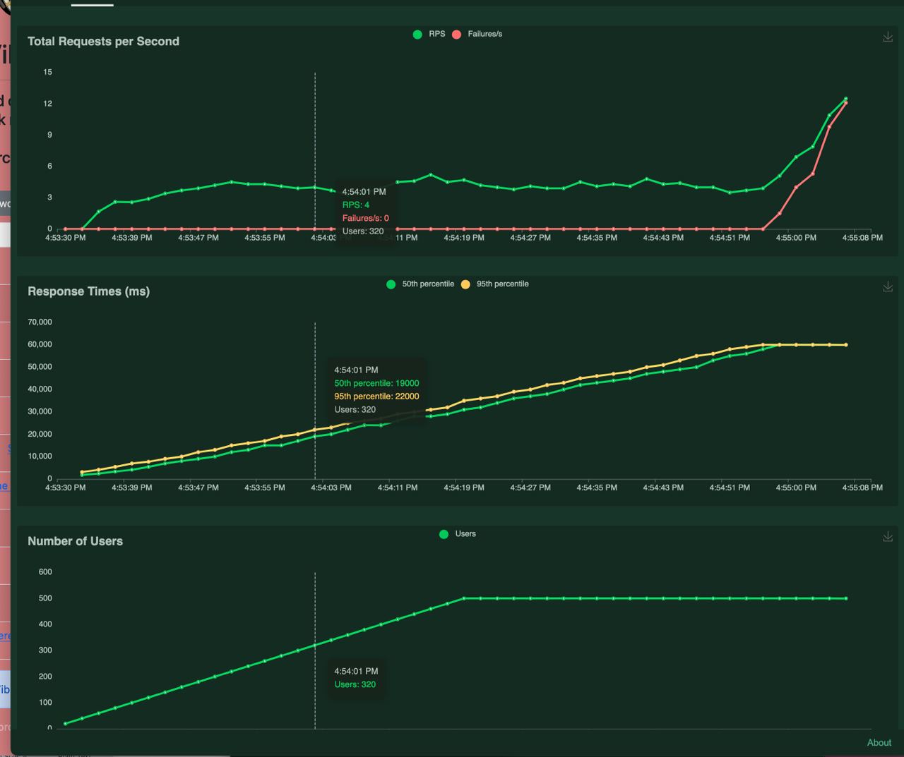
- Locust for load testing
- a logging module for capturing queries and outputs
- and tests in pytest
Tooling
- PyCharm for development, including in Docker via bind mounts
- iterm2
- VSCode for specifically writing the documentation, it’s nicer than PyCharm for this
- Whimsical for charts
- Docker Desktop for Mac (considered briefly switching to Podman but haven’t yet)
Training Data
The original book data comes from UCSD Book Graph, which scraped it from Goodreads for research papers in 2017-2019.
The data is stored in several gzipped-JSON files:
- books - detailed meta-data about 2.36M books
- reviews - Complete 15.7m reviews (~5g):15M records with detailed review text
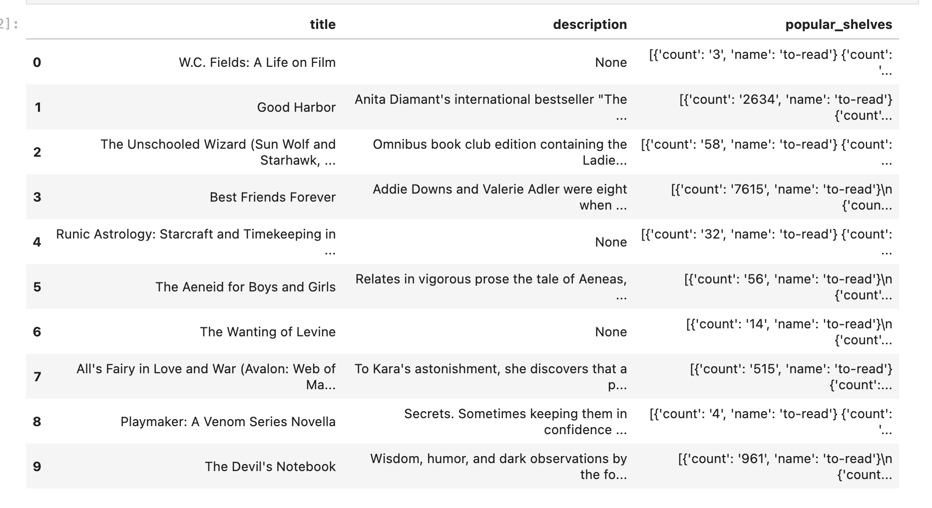
Sample row: Note these are all encoded as strings!
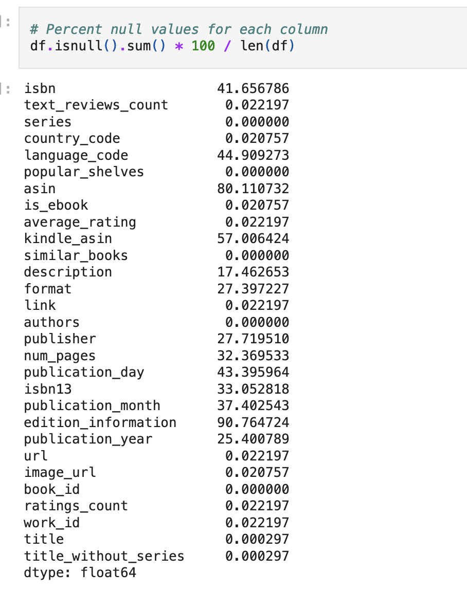
There is a lot of good stuff in this data! So, like any good data scientist, I initially did some data exploration to get a feel for the data I had at hand. I wanted to know how full the dataset was, how many missing data I had, what language most of the reviews are in, and other things that will help understand what the model’s embedding space looks like.
The data input generally looks like this:
Then, I constructed several tables that I’d need to send to the embeddings model to generate embeddings for the text. I did this all in DuckDB. The final relationships between the tables look like this:
The sentence column which concatenates review_text || goodreads_auth_ids.title || goodreads_auth_ids.description is the most important because it’s this one that is used as a representation of the document to the embedding model and the one we use to generate numerical representations and look up similarity between the input vector.
There are a couple of things to note about the data. First, it’s from 2019 so the recency on the recommendations from the data won’t be great, but it should do fairly well on classical books. Second, since Goodreads no longer has an API, it’s impossible to get this updated in any kind of reasonable way. It’s possible that future iterations of Viberary will use something like Open Library, but this will involve a lot of foundational data work. Third, there is a strong English-language bias in this data, which means we might not be able to get good results in other languages at query time if we want to make Viberary international.
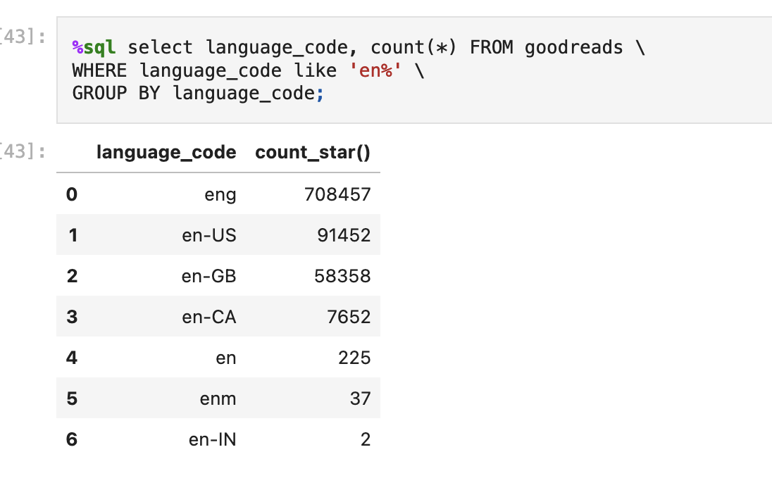
Finally, in looking at the data available per column, it looks like we have a pretty full set of data available for author, title, ratings, and description (lower percent means less null values per column) which means we’ll be able to use most of our data for representing the corpus as embeddings.
The Model
If you want to understand more of the context behind this section, read my embeddings paper.
Viberary uses Sentence Transformers, a modified version of the BERT architecture that reduces computational overhead for deriving embeddings for sentence pairs in a much more operationally efficient way than the original BERT model, making it easy to generate sentence-level embeddings that can be compared relatively quickly using cosine similarity.
This fits our use case because our input documents are several sentences long, and our query will be a keyword like search of at most 10 or 11 words, much like a short sentence.
BERT stands for Bi-Directional Encoder and was released 2018, based on a paper written by Google as a way to solve common natural language tasks like sentiment analysis, question-answering, and text summarization. BERT is a transformer model, also based on the attention mechanism, but its architecture is such that it only includes the encoder piece. Its most prominent usage is in Google Search, where it’s the algorithm powering surfacing relevant search results. In the blog post they released on including BERT in search ranking in 2019, Google specifically discussed adding context to queries as a replacement for keyword-based methods as a reason they did this. BERT works as a masked language model, which means it works by removing words in the middle of sentences and guessing the probability that a given word fills in the gap. The B in Bert is for bi- directional, which means it pays attention to words in both ways through scaled dot-product attention. BERT has 12 transformer layers. It uses WordPiece, an algorithm that segments words into subwords, into tokens. To train BERT, the goal is to predict a token given its context, or the tokens surrounding it.
The output of BERT is latent representations of words and their context — a set of embeddings. BERT is, essentially, an enormous parallelized Word2Vec that remembers longer context windows. Given how flexible BERT is, it can be used for a number of tasks, from translation, to summarization, to autocomplete. Because it doesn’t have a decoder component, it can’t generate text, which paved the way for GPT models to pick up where BERT left off.
However, this architecture doesn’t work well for parallelizing sentence similarity, which is where sentence-transformers comes in.
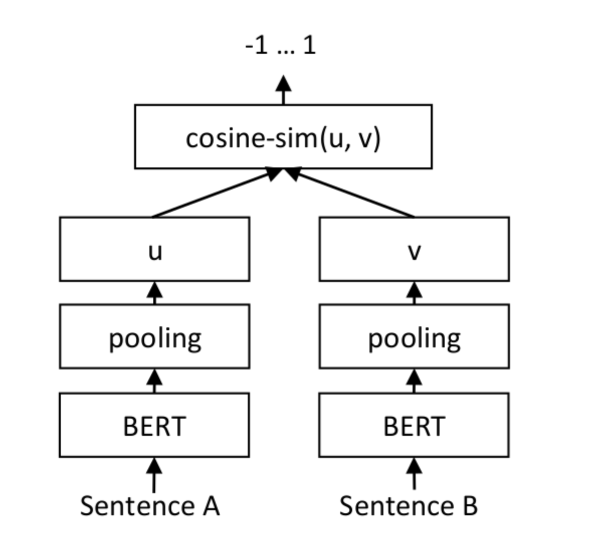
Given a sentence, a, and a second sentence, b, from an input, upstream model with BERT or similar variations as its source data and model weights, we’d like to learn a model whose output is a similarity score for two sentences. In the process of generating that score, the intermediate layers of that model give us embeddings for subsentences and words that we can then use to encode our query and corpus and do semantic similarity matching.
Given two input sentences, we pass them through the sentence transformer network and uses mean-pooling (aka averaging) all the embeddings of words/subwords in the sentence, then compares the final embedding using cosine similarity, a common distance measure that performs well for multidimensional vector spaces
Sentence Transformers has a number of pre-trained models that are on this architecutre, the most common of which is sentence-transformers/all-MiniLM-L6-v2, which maps sentences and paragraphs into a 384-dimension vector space. This means that each sentence is encoded in a vector of 384 values.
The initial results of this model were just so-so, so I had to decide whether to use a different model or tune this one. The different model I considered was the series of MSMarco models , which were trained based on sample Bing searches. This was closer to what I wanted. Additionally, the search task was asymmetric, which meant that the model accounted for the fact that the corpus vector would be longer than the query vector.
I chose msmarco-distilbert-base-v3, which is middle of the pack in terms of performance, and critically, is also tuned for cosine similarity lookups, instead of dot product, another similarity measure that takes into account both magnitude and direction. Cosine similarity only considers direction rather than size, making cosine similarity more suited for information retrieval with text because it’s not as affected by text length, and additionally, it’s more efficent at handling sparse representations of data.
There was a problem, however, because the vectors for this series of models was twice as long, at 768 dimensions per embedding vector. The longer a vector is, the more computationally intensive it is to work with, increasing, with the runtime and the memory requirement grows quadratic with the input length. However, the longer it is, the more information about the original input it compresses, so there is always a fine-lined tradeoff between being able to encode more information and faster inference, which is critical in search applications.
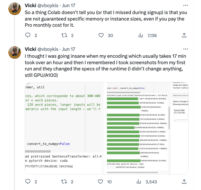
Learning embeddings was tricky not only in selecting the correct model, but also because everyone in the entire universe is using GPUs right now.
I first tried Colab, but soon found that, even at the paid tier, my instances would mysteriously get shut down or downgraded, particularly on Friday nights, when everyone is doing side projects.
I then tried Paperspace but found its UI hard to navigate, although, ironically, recently it’s been purchased by Digital Ocean which I always loved and have become even more a fan of over the course of this project. I settled on doing the training on AWS since I already have an account and, in doing PRs for PyTorch, had already configured EC2 instances for deep learning.
The process turned out to be much less painless than I anticipated, with the exception that P3 instances run out very quickly due to everyone training on them. But it only took about 20 minutes to generate embeddings for my model, which is a really fast feedback loop as far as ML is concerned. I then wrote that data out to a snappy-compressed parquet file that I then load manually to the server where inference is performed.
Redis and Indexing
Once I learned embeddings for the model, I needed to store them somewhere for use at inference time. Once the user inputs a query, that query is transformed also into an embedding representation using the same model, and then the KNN lookup happens. There are about five million options now for storing embeddings for all kinds of operations.
Some are better, some are worse, it all depends on your criteria. Here were my criteria:
- an existing technology I’d worked with before
- something I could host on my own and introspect
- something that provided blazing-fast inference
- a software package where the documentation tells you
O(n)performance time of all its constitutent data structures
I’m kidding about the last one but it’s one of the things I love about the Redis documentation. Since I’d previously worked with Redis as a cache, already knew it to be highly reliable and relatively simple to use, as well as plays well with high-traffic web apps and available packaged in Docker, which I would need for my next step to production, I went with Redis Search, which offers storage and inference out of the box, as well as frequently updated Python modules.
Redis Search is an add-on to Redis that you can load as part of the redis-stack-server Docker image.
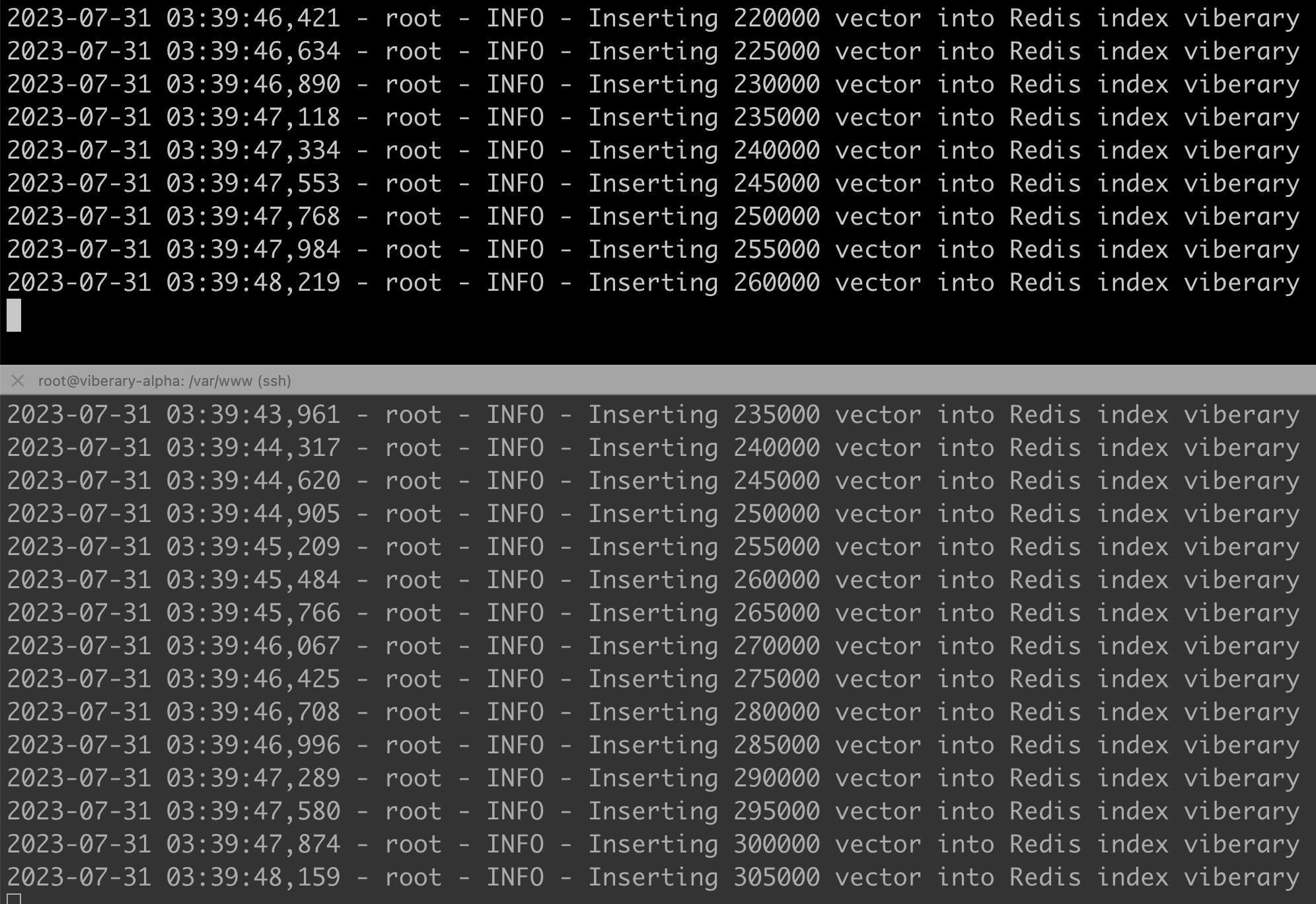
It offers vector similarity search by indexing vectors stored as fields in Redis hash data structures, which are just field-value pairs like you might see in a dictionary or associative array. The common Redis commands for working with hashes are HSET and HGET, and we can first HSET our embeddings and then create an index with a schema on top of them. An important point is that we only want to create the index schema after we HSET the embeddings, otherwise performance degrades significantly.
For our learned embeddings which encompass ~800k documents, this process takes about ~1 minute.
Lookups and Request/Response
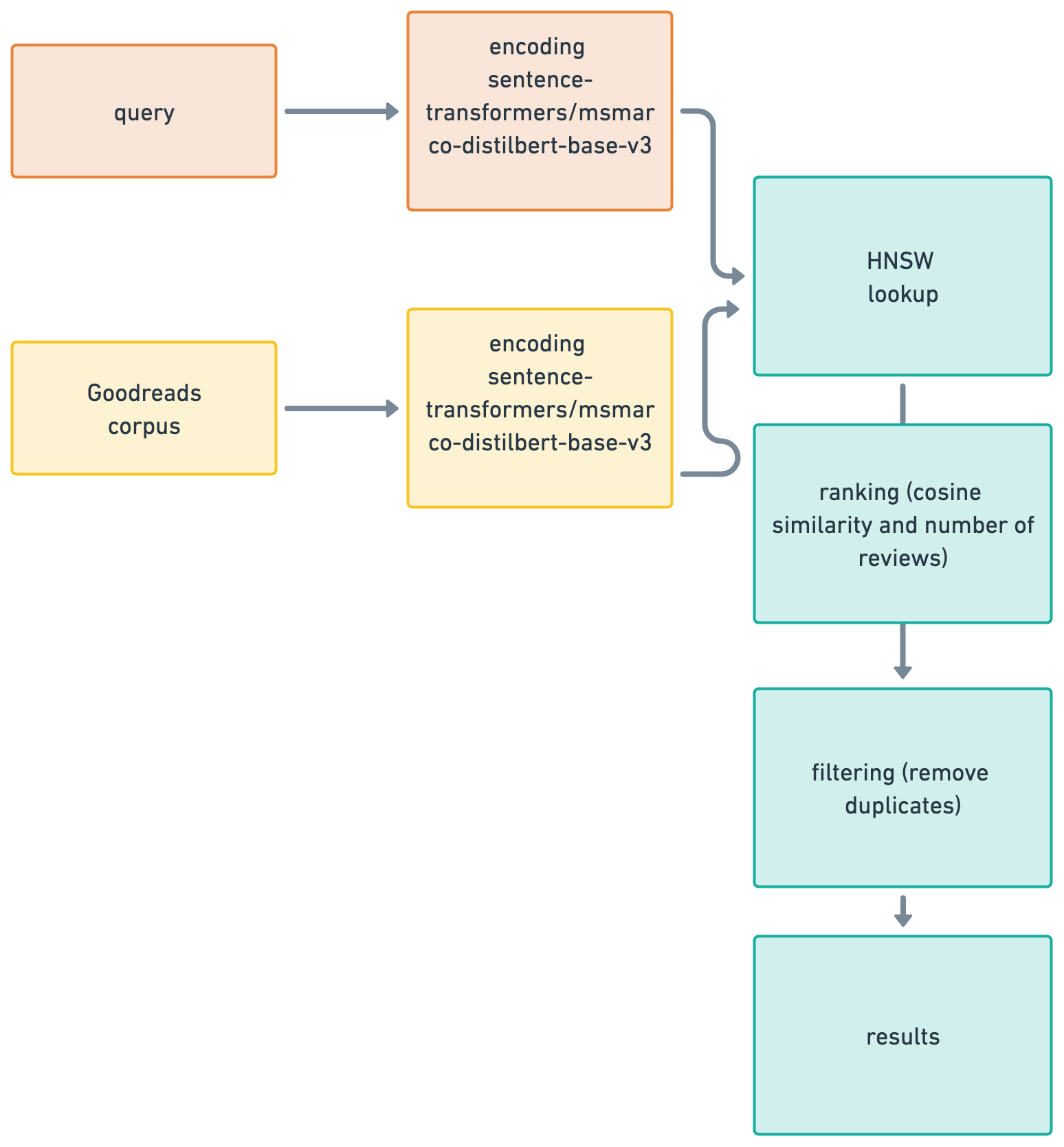
Now that we have the data in Redis, we can perform lookups within the request-response cycle. The process looks like this:
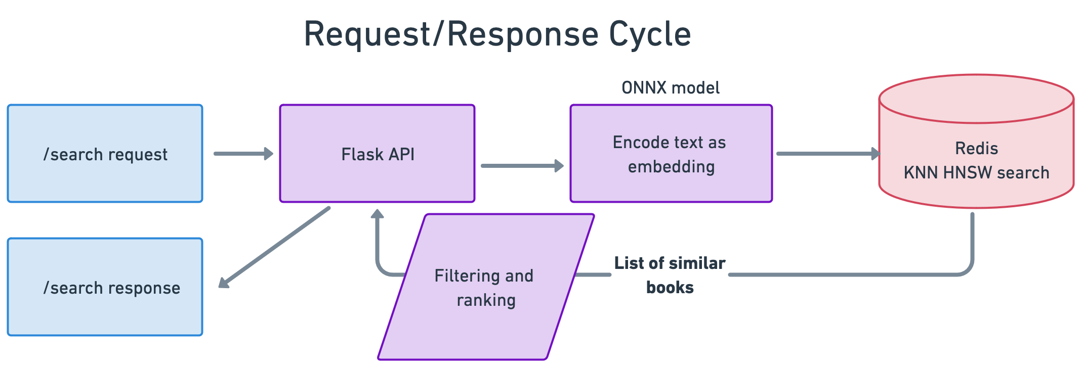
Since we’ll be doing this in the context of a web app, we write a small Flask application that has several routes and captures the associated static files of the home page, the search box, and images, and takes a user query, runs it through the created search index object after cleaning the query, and returns a result:
that data gets passed into the model through a KNN Search object which takes a Redis connection and a config helper object:
The search class is where most of the real work happens. First, the user query string is parsed and sanitized, although in theory, in BERT models, you should be able to send the text as-is, since BERT was originally trained on data that does not do text clean-up and parsing, like traditional NLP does.
Then, that data is rewritten into the Python dialect for the Redis query syntax. The search syntax is can be a little hard to work with originally, both in the Python API and on the Redis CLI, so I spent a lot of time playing around with this and figuring out what works best, as well as tuning the hyperparameters passed in from the config file, such as the number of results, the vector size, and the float type (very important to make sure all these hyperparameters are correct given the model and vector inputs, or none of this works correctly.)
HNSW is the algorithm, initially written at Twitter, implemented in Redis that actually peforms the query to find approximate nearest neighbors based on cosine similarity. It looks for an approximate solution to the k-nearest neighbors problem by formulating nearest neighbors as a graph search problem to be able to find nearest neighbors at scale. Naive solutions here would mean comparing each element to each other element, a process which computationally scales linearly with the number of elements we have. HNSW bypasses this problem by using skip list data structures to create multi-level linked lists to keep track of nearest neighbors. During the navigation process, HNSW traverses through the layers of the graph to find the shortest connections, leading to finding the nearest neighbors of a given point.
It then returns the closest elements, ranked by cosine similarity. In our case, it returns the document whose 768-dimension vector most closely matches the 768-dimension vector generated by our model at query time.
The final piece of this is filtering and ranking. We sort by cosine similarity descending, but then also by the number of reviews - we want to return not only books that are relevant to the query, but books that are high-quality, where number of reviews is (questionably) a proxy for the fact that people have read them. If we wanted to experiment with this, we could return by cosine similarity and then by nubmer of stars, etc. There are numerous ways to fine-tune.
Getting the UI Right
Once we get the results from the API, we get back is a list of elements that include the title, author, cosine similarity, and link to the book. It’s now our job to present this to the user, and to give them confidence that these are good results. Additionally, the results should be able to prompt them to build a query.
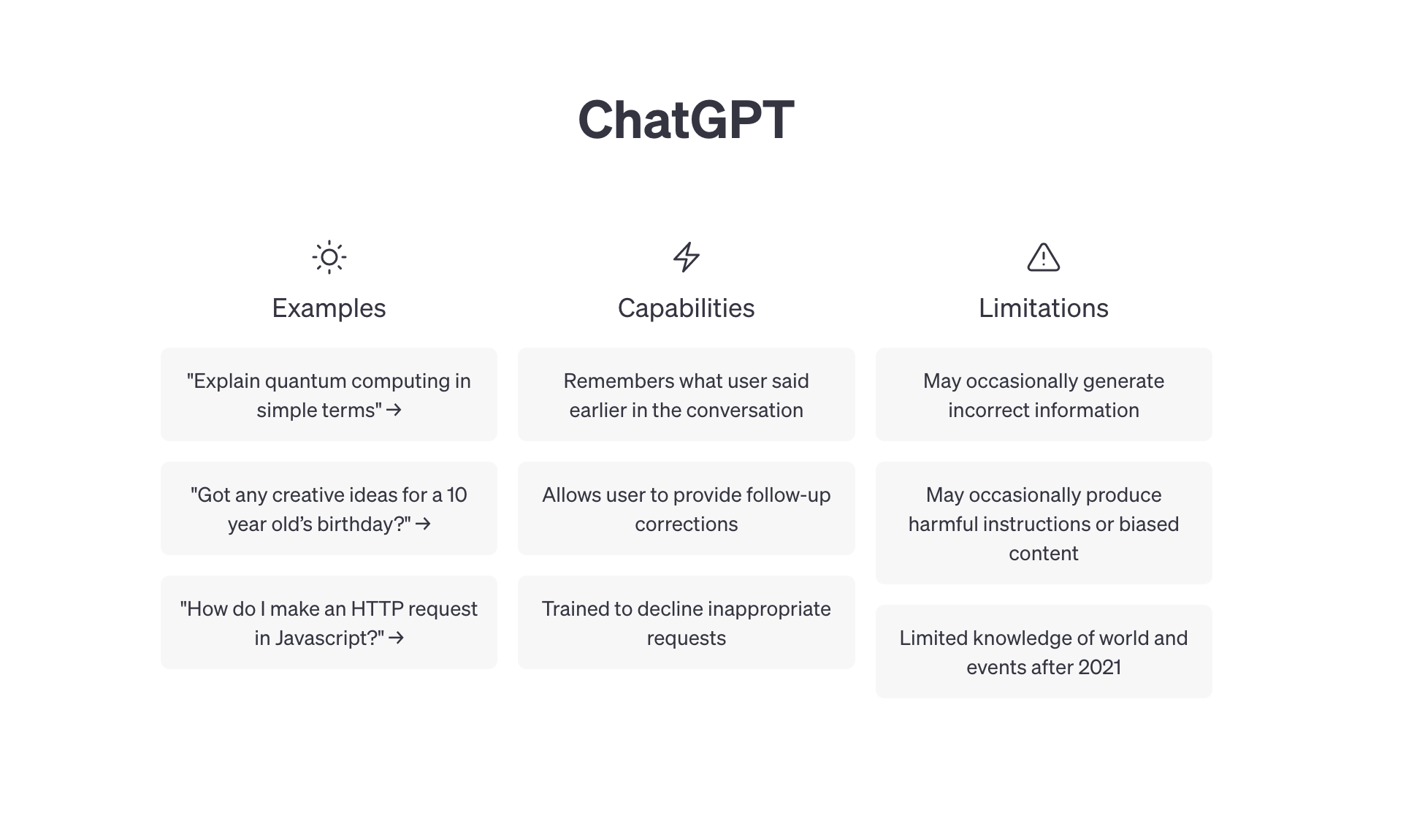
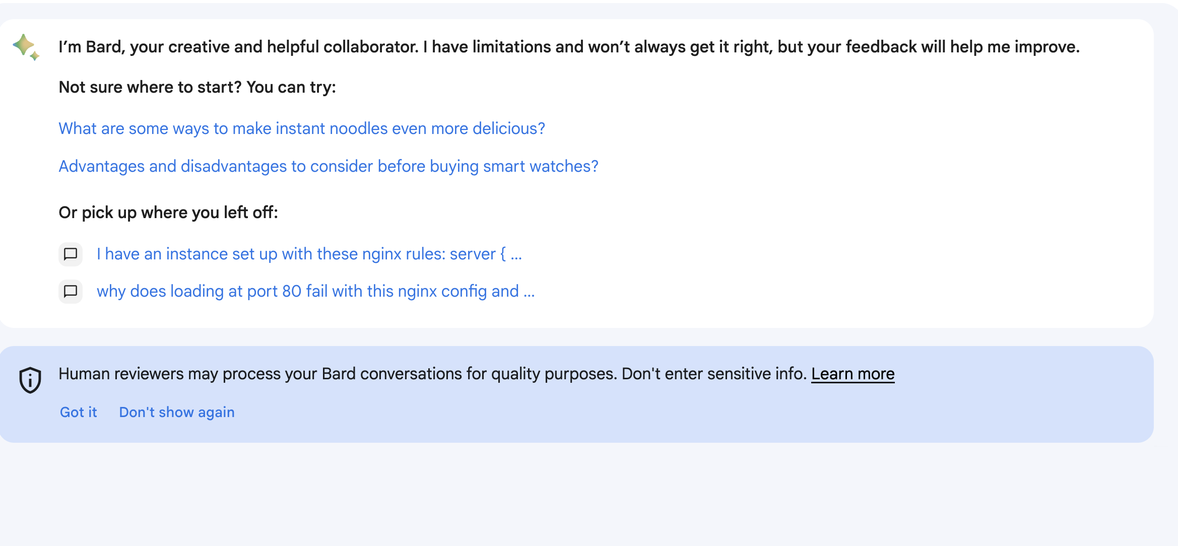
Research has found, and perhaps your personal experience has proven, that it’s hard to stare into a text box and know what to search for, particularly if the dataset is new to you. Additionally, the UX of the SERP page matters greatly. That’s why generative AI products, such as Bard and OpenAI often have prompts or ideas of how to use that open-ended search box.
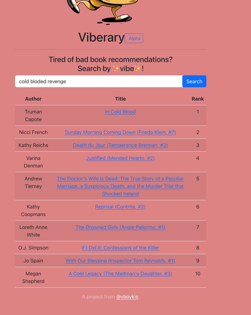
The hard part for me was in getting users to understand how to write a successful vibe query that focused on semantic rather than direct search. I started out with a fairly simple results page that had the title and the rank of the results.
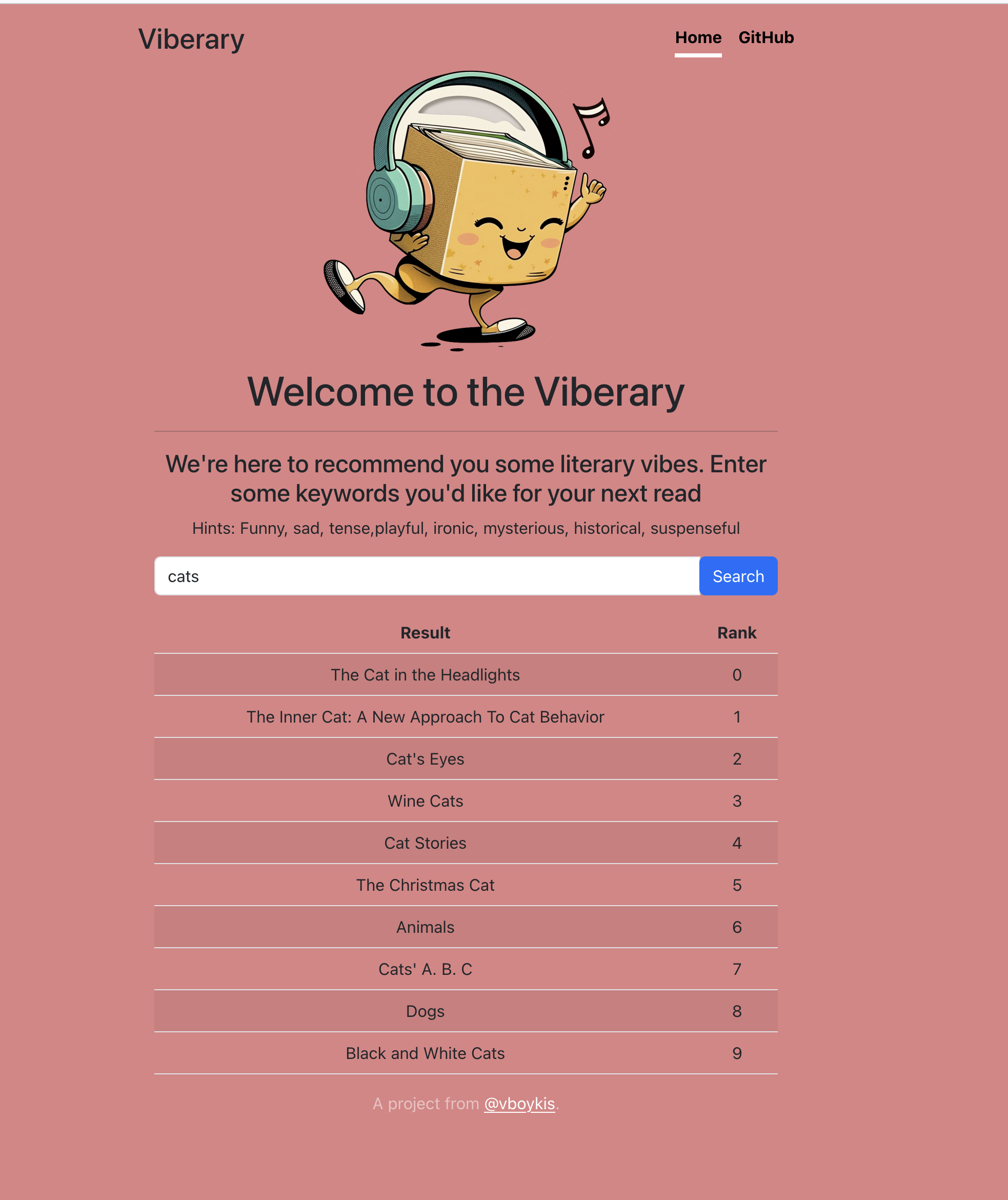
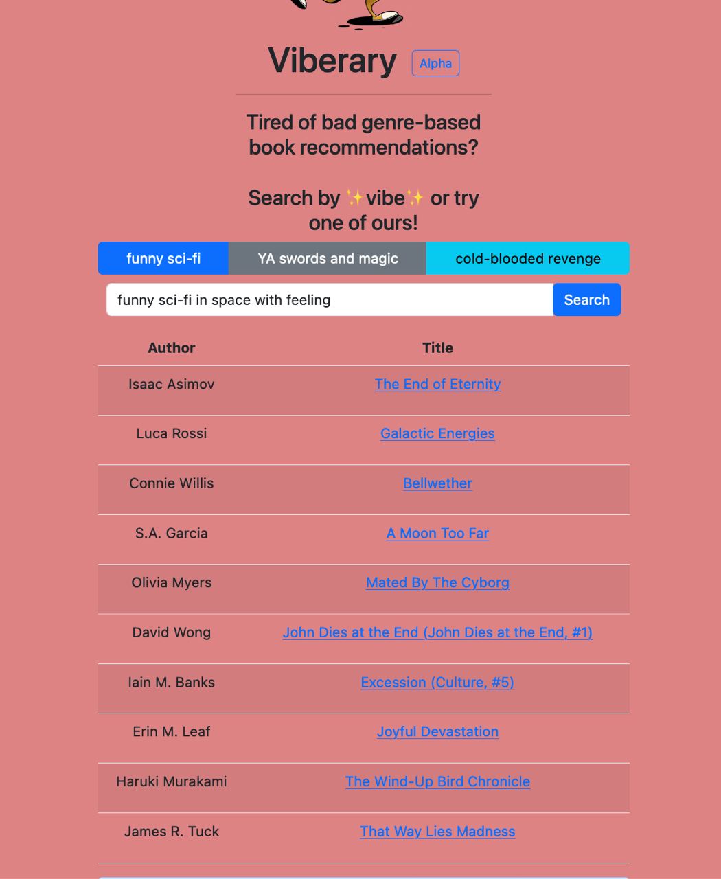
It became clear that this was not satisfactory: there was no way to reference the author or to look up the book, and the ranking was confusing, particularly to non-developers who were not used to zero indexing. I then iterated to including the links to the books so that people could introspect the results.
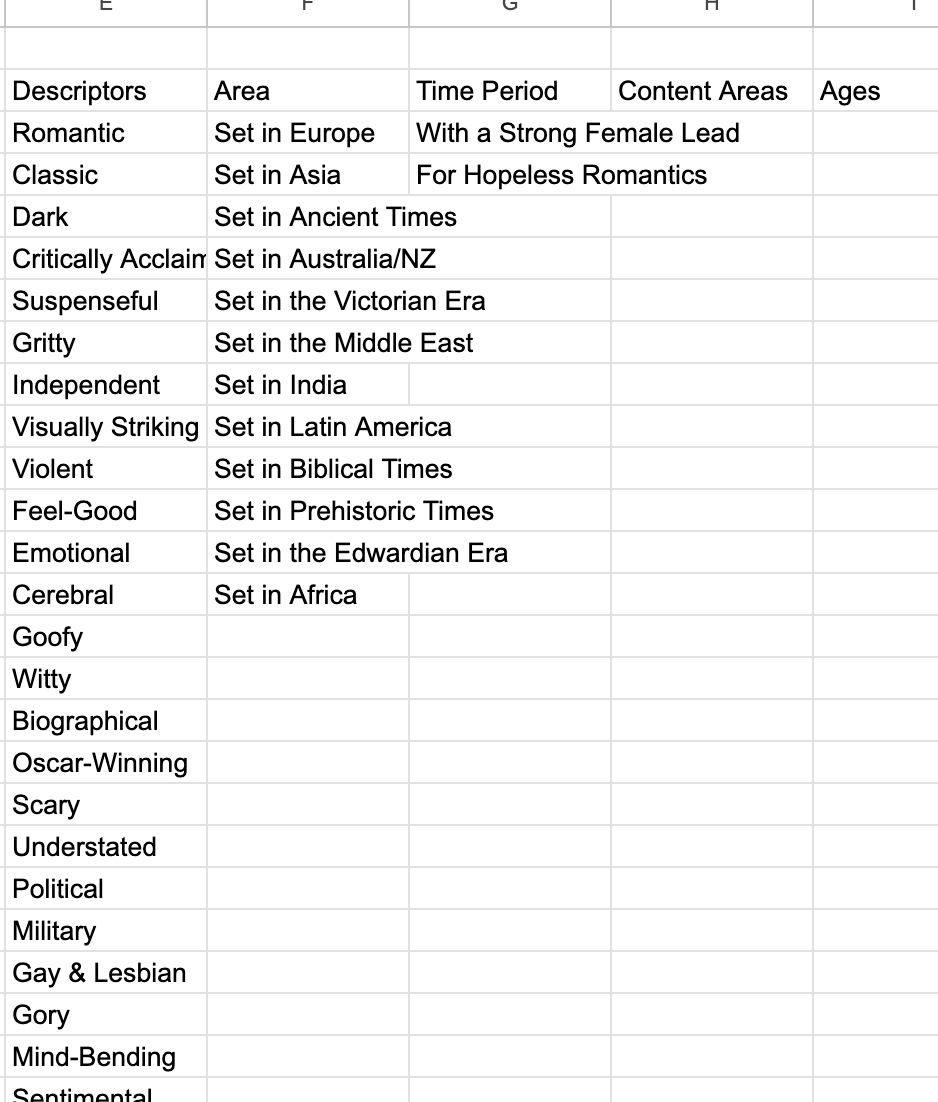
I removed the ranking because it felt more confusing and took up more computational power to include it, and additionally people generally understand that best search results are at the top. Finally, I added button suggestions for types of queries to write. I did this by looking at the list of Netflix original categories to see if I could create some of my own, and also by asking friends who had tested the app.
On top of all of this, I worked to make the site load quickly both on web and mobile, since most people are mobile-first when accessing sites in 2023. And finally, I changed the color to a lighter pink to be more legible. This concludes the graphic design is my passion section of this piece.
DigitalOcean, Docker, and Production
Now that this all worked in a development environment, it was time to scale it for production. My top requirements included being able to develop locally quickly and reproduce that environment almost exactly on my production instances, a fast build time for CI/CD and for Docker images, the ability to horizontally add more nodes if I needed to but not mess with autoscaling or complicated AWS solutions, and smaller Docker images than is typical for AI apps, which can easily balloon to 10 GB with Cuda GPU-based layers.. Since my dataset is fairly small and the app itself worked fairly well locally, I decided to stick with CPU-based operations for the time being, at least until I get to a volume of traffic where it’s a problem.
Another concern I had was that, halfway through the project (never do this), I got a new Macbook M2 machine, which meant a whole new world of pain in shipping code consistently between arm and intel architectures.
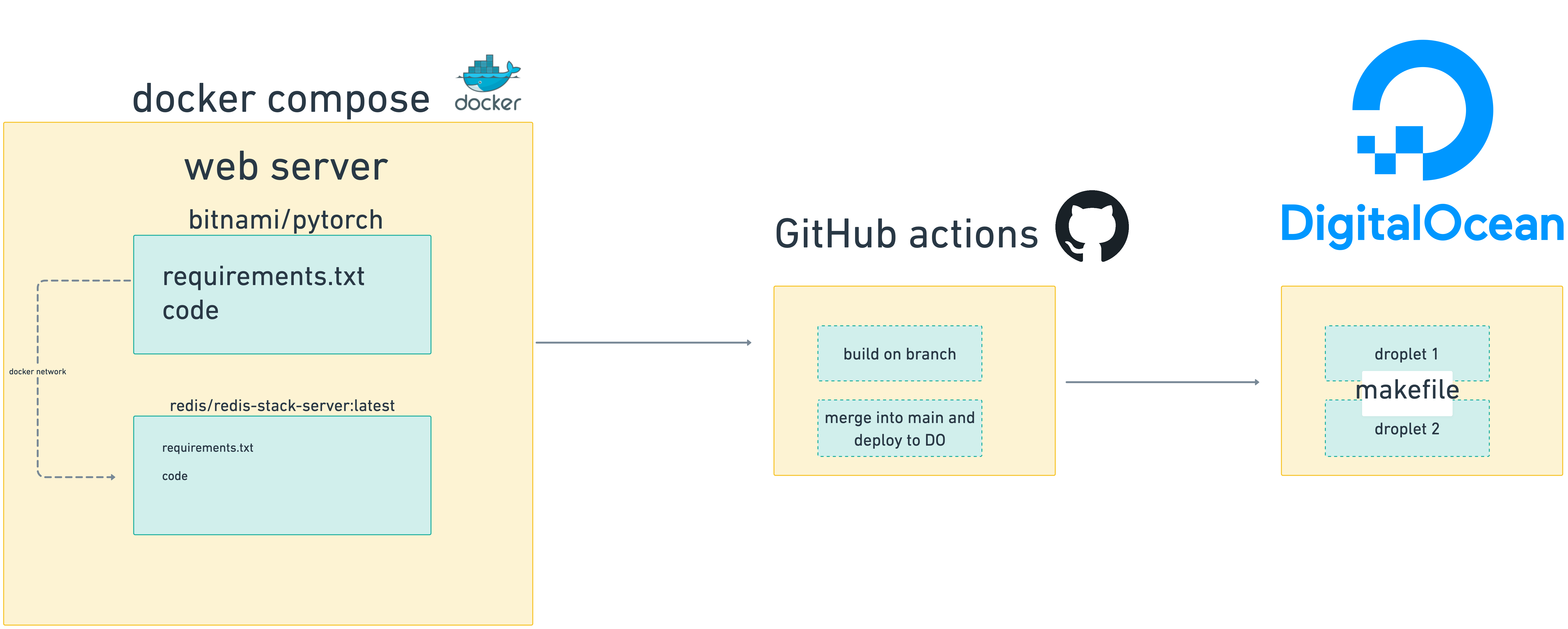
My deployment story works like this. The web app is developed in a Docker container that I have symlinked via bind mounts to my local directory so that I write code in PyCharm and changes are reflected in the Docker container. The web docker container is networked to Redis via Docker’s internal network. The web app is available at 8000 on the host machine, and, in production in Nginx, proxies port 80 so we can reach the main domain without typing in ports and hit Viberary. In the app dockerfile, I want to make sure to have the fastest load time possible, so I follow Docker best practices of having the layers that change the most last, caching, and mounting files into the Docker image so I’m not constantly copying data.
The docker image base for the web is bitnami:pytorch and it installs requirements via requirements.txt
I have two Dockerfiles, one local and one for production. The production is linked from the docker-compose file and correctly builds on the Digital Ocean server. The local one is linked from the docker-compose.override file, which is excluded from version control, but which works only locally, so that each environment gets the proper build directives.
├── docker
│   ├── local
│   │   └── Dockerfile
│   └── prod
│       └── Dockerfile
├── docker-compose.override.yml
├── docker-compose.yml
The Docker compose takes this Dockerfile and networks it to the Redis container.
All of this is run through a Makefile that has commands to build, serve, spin down, and run onnx model creation from the root of the directory. Once I’m happy with my code, I push a branch to GitHub where github actions runs basic tests and linting on code that should, in theory, already be checked since I have precommit set up. The pre-commit hook lints it and cleans everything up, including black, ruff, and isort, before I even push to a branch.
Then, once the branch passes, I merge into main. The main branch does tests and pushes the latest git commit to the Digital Ocean server. I then manually go to the server, bring down the old docker image and spin up the new one, and the code changes are live.
Finally, on the server, I have a very scientific shell script that helps me configure each additional machine. Since I only needed to do two, it’s fine that it’s fairly manual at the moment.
Finally everything is routed to port 80 via nginx, which I configured on each DigitalOcean droplet that I created. I load balanced two droplets behind a load balancer, pointing to the same web address, a domain I bought from Amazon’s Route 53. I eventually had to transfer the domain to Digital Ocean, because it’s easier to manage SSL and HTTPS on the load balancer when all the machines are on the same provider.
Now, we have a working app. The final part of this was load testing, which I did with Python’s Locust library, which provides a nice interface for running any type of code against any endpoint that you specify. One thing that I realized as I was load testing was that my model was slow, and search expects instant results, so I converted it to an ONNX artifact and had to change the related code, as well.
Finally, I wrote a small logging module that propogates across the app and keeps track of everything in the docker compose logs.
Key Takeaways
Getting to a testable prototype is key. I did all my initial exploratory work locally in Jupyter notebooks, including working with Redis, so I could see the data output of each cell. I strongly believe working with a REPL will get you the fastest results immediately. Then, when I had a strong enough grasp of all my datatypes and data flow, I immediately moved the code into object-oriented, testable modules. Once you know you need structure, you need it immediately because it will allow you to develop more quickly with reusable, modular components.
Vector sizes and models are important. If you don’t watch your hyperparameters, if you pick the wrong model for your given machine learning task, the results are going to be bad and it won’t work at all.
Don’t use the cloud if you don’t have to. I’m using DigitalOcean, which is really, really, really nice for medium-sized companies and projects and is often overlooked over AWS and GCP. I’m very versant in cloud, but it’s nice to not have to use BigCloud if you don’t have to and to be able to do a lot more with your server directly. DigitalOcean has reasonable pricing, reasonable servers, and a few extra features like monitoring, load balancing, and block storage that are nice coming from BigCloud land, but don’t overwhlem you with choices. They also recently acquired Paperspace, which I’ve used before to train models, so should have GPU integration.
DuckDB is becoming a stable tool for work up to 100GB locally. There are a lot of issues that still need to be worked out because it’s a growing project. For example, for two months I couldn’t use it for my JSON parsing because it didn’t have regex features that I was looking for, which were added in 0.7.1, so use with caution. Also, since it’s embedded, you can only run one process at a time which means you can’t run both command line queries and notebooks. But it’s a really neat tool for quickly munging data.
Docker still takes time I spent a great amount of time on Docker. Why is Docker different than my local environment? How do I get the image to build quickly and why is my image now 3 GB? What do people do with CUDA libraries (exclude them if you don’t think you need them initially, it turns out). I spent a lot of time making sure this process worked well enough for me to not get frustrated rebuilding hundreds of times. Relatedly, Do not switch laptop architectures in the middle of a project .
Deploying to production is magic, even when you’re a very lonely team of one, and as such is filled with a lot of unknown variables, so make your environments as absolutely reproducible as possible.
And finally,
- True semantic search is very hard and involves a lot of algorithmic fine-tuning, both in the machine learning, and in the UI, and in deployment processes. People have been fine-tuning Google for years and years. Netflix had thousands of labelers. Each company has teams of engineers working on search and recommendations to steer the algorithms in the right direction. Just take a look at the company formerly known as Twitter’s algo stack. It’s fine if the initial results are not that great.
The important thing is to keep benchmarking the current model against previous models and to keep iterating and keep on building.
Citations
Resources
- Relevant Search by Turnbull and Berryman
- Corise Search Course and Search with Machine Learning - I’ve taken these, and have nothing to sell except the fact that Grant and Daniel are aweosme. Code is here.
- What Are Embeddings - during the process of writing this I came up with a lot of sources included in the site and bibliography
- Towards Personalized and Semantic Retrieval: An End-to-End Solution for E-commerce Search via Embedding Learning
- Pretrained Transformers for Text Ranking: BERT and Beyond
- Advanced IR Youtube Series