What's new with ML in production

In 2023, I wrote two pieces on machine learning engineering for The Pragmatic Programmer. (Part 1 and Part 2). However, since I started working with LLMs recently, neural architectures have changed some of those assumptions.
To be clear, most of machine learning in production is still not related to large language models or generative AI, and even deep learning projects, of which LLMs are a small subset, make up no more than 10% of the market, at most. But it’s still helpful to compare and contrast classical ML systems with their LLM counterparts, because this is where we’re going in the future.
Machine learning is compression
At its core, a machine learning model is an algorithm that performs compression on a corpus of data.

In the first half of the 20th century, when digital communication in the then-nascent telephone industry exploded, scientists and engineers at Bell Labs started studying the projection and representation of information. In developing this field, scientists like Harry Nyquist, Ralph Hartley, and Claude Shannon were concerned with irregularities in information transfer, particularly across radio signals . Information theory was developed to solve the problem of transmitting a message, via radio, telephone, or television, with the most accuracy. It turned out that the most efficient way to inspect information was to not look at the actual data, but to analyze the statistical properties of that message. So, much of the science work centered around creating approximate representations of data. For example, Kolmogorov complexity, was developed as an notion that describes how much information is needed to represent something. In the case of a string, it’s the shortest program that can generate that string. The more complex that string is, the higher specification a program.
What came out of the early work in information theory was that, in order to efficiently work with large amounts of information, we need to be able to effectively compress it into as little space as we can without losing fidelity of that information.
Given the continued explosion of text, and later multi-modal (voice, video, etc.) information, the algorithms developed around compression continued to stay relevant. Compression is the same fundamental concept underlying both traditional machine learning models and LLMs, although this idea is usually burried under layers of other context.

GZip is compression is machine learning
Every once in a while, this initial context comes out. For example, a few months ago, a paper came out that took the machine learning world by storm. With the unassuming title, “Less is More: Parameter-Free Text Classification with Gzip”, the paper claimed that simply compressing data using gzip and running knn search over the compressed data for classification tasks beats gold-standard neural network-based language models like BERT.
The premise behind the work was that is that in any given collection of objects, we can compare them based on how close they are to each other, and for the downstream task, classify them in categories, in a way that doesn’t involve deep learning.
For example, let’s say we have a dataset of news article headlines., and we have several categories of headlines (business, sports, tech, and more). The data looks like this:
{
    "label": 2,
    "text": "Stocks End Up, But Near Year Lows (Reuters) Reuters - Stocks ended slightly higher on Friday but stayed near lows for the year as oil prices surged past a barrel, offsetting a positive outlook from computer maker Dell Inc. (DELL.O)"
}
Given a new headline, can we learn some kind of model that will accurately match the string to a category? We might want to do this for any number of reasons: assigning trending topics in a site like Flutter, categorizing items in ecommerce for sale, or knowledge curation within companies, or within medicine.
How might we do this if we have to brute force it? We’d take a string and compare it, character by character, to another string. That’s the idea behind Levenshtein, or edit, distance.. This approach means you quickly start running into problems where you have to perform O(N) lookups across your entire dataset and have to start keeping track of data in lists or arrays.
We might then use traditional methods like TF-IDF to classify the strings. This also eventually runs into scaling issues as your vocabulary size becomes bigger and bigger. More often recently, neural network and deep learning approaches like BERT, and even more recently, autoregressive models like those in the GPT family are being used for classification tasks.
However, once we start using deep learning models, we run into arrays and dictionaries that become larger and larger; i.e. matrix math, which means we need GPUs and extremely large datasets. Is there any way we can work around this to create representations of our strings that are not the actual string that allow us to work with shorthand versions of our original information? For example, it would be great if, instead of having to compare these two strings:
Stocks End Up, But Near Year Lows (Reuters) Reuters - Stocks ended slightly higher on Friday but stayed near lows for the year as oil prices surged past a barrel, offsetting a positive outlook from computer maker Dell Inc. (DELL.O)
Money Funds Fell in Latest Week (AP) AP - Assets of the nation's retail money market mutual funds fell by #36;1.17 billion in the latest week to $849.98 trillion, the Investment Company Institute said Thursday.
We could compare something like a numerical representation of the strings and see if they’re similar. We could learn embeddings which would take time, but what if we go simpler? What’s a function that compresses information? Gzip does. (Code examples duplicated for clarity.)
import gzip
import io
input_string = """Stocks End Up, But Near Year Lows (Reuters) Reuters -
Stocks ended slightly higher on Friday
but stayed near lows for the year as oil prices surged past a barrel,
offsetting a positive outlook from computer maker Dell Inc. (DELL.O)"""

input_bytes = input_string.encode('utf-8')

output_buffer = io.BytesIO()

compressed_data = output_buffer.getvalue()
print(compressed_data)
b'\x1f\x8b\x08\x00\xdd\xaa\x8de\x02\xff%\x8dM\x0b\x82@\x14E\xf7\xfe\x8a\xbb\x08*(A\x08\xd2\xa5\x04BP\xe0"h=\xe2\x13\x07\xe7#|o\x8a\xf9\xf79\xba\xbd\x9c{\xce\xd3;\x8ah\x82\xeb\x19\r\x19\x03\xed\xf0PB,x\x13M8\xd4\xed\x11u\x8b3\xb2\x9a\x99\x84\xe1\x07\xc8HpJ\xb4w{\xc6L\xa2\xb4\x81]EV\xcd\x13\tl\x90\xa0\x0c\x86U;$m\x17\x91\xed\x8a\xbc\xb8\xa2\xd3\xc6,\xcf\x14J\x1e\xb3\xc5~)&\x1e\xbb\xf2R\xe5U\t\x997\xec\x84,Qw\xf7](KNp\xf3\xf6\xa3\\\\&\x16-A\x08\xact\x8f\xd7\x18f\xeeU\xcc\xff\x17\xe6\xe7v\xd2\x00\x00\x00'
import gzip
import io
input_string = """Money Funds Fell in Latest Week (AP) AP -
Assets of the nation's retail money market mutual funds fell by
$1.17 billion in the latest week to $849.98 trillion,
the Investment Company Institute said Thursday."""

input_bytes = input_string.encode('utf-8')

output_buffer = io.BytesIO()

compressed_data = output_buffer.getvalue()
print(compressed_data)
b'\x1f\x8b\x08\x00\xdd\xaa\x8de\x02\xff%\x8dM\x0b\x82@\x14E\xf7\xfe\x8a\xbb\x08*(A\x08\xd2\xa5\x04BP\xe0"h=\xe2\x13\x07\xe7#|o\x8a\xf9\xf79\xba\xbd\x9c{\xce\xd3;\x8ah\x82\xeb\x19\r\x19\x03\xed\xf0PB,x\x13M8\xd4\xed\x11u\x8b3\xb2\x9a\x99\x84\xe1\x07\xc8HpJ\xb4w{\xc6L\xa2\xb4\x81]EV\xcd\x13\tl\x90\xa0\x0c\x86U;$m\x17\x91\xed\x8a\xbc\xb8\xa2\xd3\xc6,\xcf\x14J\x1e\xb3\xc5~)&\x1e\xbb\xf2R\xe5U\t\x997\xec\x84,Qw\xf7](KNp\xf3\xf6\xa3\\\\&\x16-A\x08\xact\x8f\xd7\x18f\xeeU\xcc\xff\x17\xe6\xe7v\xd2\x00\x00\x00'
Now that we’ve compressed the strings into compact representations, we can then compare these representations. (see the original paper implementation here) The gzip paper suggested that compressing two pieces of similar text using any given simple compression method, will result in similar pieces of text having more similar size in bytes than dissimilar pieces. This means that we can rank and compare representations by their similarity, as well as label them.
Then, to create the label, the most common label among the k reference texts with the lowest normalized compression distance scores is the label of the text.
The authors of the paper claimed that this method beat out BERT, mBERT, fastText, and word2vec. Naturally, there was some skepticism around this, and in performing tests, the community found that the offline evaluation metrics the authors were using to compute accuracy were not standard (i.e. they gave more leniency in selecting either of the top two options rather than making sure that the top option was the best.)
Machine learning tasks as compression
There was a lot of conversation around this paper, and then everyone forgot it in the breakneck pace of LLM model development that followed. The main takeaway is that compression is the core of machine learning. As long as we want to condense some given state of the world and try to generalize from data, we need to synthesize our input data, simply because we can’t include the entire universe in service of our model.
These compression tasks take on any number of shapes: as iterative combinations of trees in gradient boosting, as user-item matrices in collaborative filtering, or as attention mechanisms in deep learning models.
The rest of machine learning is a layer of software engineering around the model artifacts to keep them working in production settings. In other words, we have the Task and the Platform.
Machine learning platforms as platforms to support compression
What are the pieces around the model? Machine learning platforms - a collection of software components that create a systematic, automated way to take raw data, transform it, learn a model from it, and show results which support decision-making for internal or external customers.
For example, Netflix’s recommendations are part of ML platform. When you call an Uber or Lyft, or book an Airbnb, the chances are you’re being served software components developed by those companies’ internal ML organizations. These are very visible, consumer end-uses of machine learning, but ML is also used in the less visible parts of ML organizations, such as fraud detection at Stripe and at banks, and in content moderation on social media platforms.
We take some given input data, learn a simplified representation of that data using a given function that we think will model the world appropriately (aka we compress), and hope that it applies to all of the data we pass into the function.

In traditional machine learning pipelines we:
ingest data about our application or its users. That data gets stored in a database or a data lake, where we process and clean it via data engineering so that we can feed it into a model. Before we can pass the data to the model, we need to ensure this data is valid and clean. To do so, we use tools like Jupyter notebooks, or the Python REPL (a command line) to quickly look at our data and iterate through it. The data’s analyzed and cleaned up as needed.
select and engineer machine learning features from that data and learn a model from those features. Features can range from “geographical location” or “number of shows watched this week”.
And then we learn a model and build the model artifacts. Model artifacts are data structures typically consisting of:
- Weights and biases. These are numbers known as the model’s parameters. Weights are numbers determining how much input influences the outputs. Biases are additional parameters which are starting points for prediction. They act as offsets and allow the model to make predictions when data is missing
- Code that describes the structure of the model, including its architecture, such as the decision tree or neural network, and the number of layers
- Dependencies and libraries the code and model use.
- Model metadata: date of training, description of the model, etc.
We perform offline evaluation of the model artifact to see if it’s any good inherently as-is. We do this by We need to answer questions like:
- Do the model’s results make statistical sense?
- Have we minimized our loss function, which is the distance between predicted and actual model results (using data we hold out as a test set)?
There are a number of different metrics to determine whether a model is “good, ” such as root mean squared error, precision, or recall. Getting these metrics usually involves feeding test data into the model that the model has not been trained on, and observing how far away the predicted value is from the actual value.
- We deploy that model to production. Deployment of those models to production, including all the associated software development components which keep models running, like monitoring, model tracking, feature tracking, dashboards, and tuning of the application’s performance.
The running model will look something like this in the context of our application:

- We then perform online evaluation of the models as we launch A/B tests and finally look at production metrics. We have now developed a feedback loop between production and our modeling cycle that enables us to update the model with new data (aka user feedback,clickstream data, changes in trends, cyclical changes) and train updated models, because data is not static, and model data is non-deterministic.
Anyone who has worked with ML systems painfully knows this is the case; often you are not only troubleshooting non-working software components: model failures can be anything from unexpected caching issues in production, a “classical” software engineering problem, or data drift which is when the properties of the model used for prediction change.
A common example of data drift is seasonality: you can’t accurately predict the same volume of ice cream sales in summer as in winter. Often, these types of drifts are not very obvious and take a long time to detect. Null or malformed log data is also a cause for “silent” modeling failures.
In addition to those components, Another property of the ML modeling process is that once you have more than one model, you’re responsible for both their input data and metadata, which means setting up additional systems to track assets, as well as changes in the system. Here’s a few examples of components in ML platforms which web apps usually don’t include:
Feature stores: functionality to pull data specifically formatted for building and serving models from the data warehouse, and do this quickly.
Monitoring data drift. Data drift occurs when input data change over time. For example, when a customer base ages. It can also happen if a new technology wasn’t included in the model’s original assumptions; for example, cell phones’ rapid spread across a telephony model built on landlines.
Model training monitoring: the goal of this is to evaluate offline performance metrics to answer questions like how well a model will perform on unseen data.
Model registries. These allow use of differently versioned model artifacts based on which is preferred for use in production.
As we can see, machine learning systems are already complex. The data-centric nature of ML means that, in addition to the usual things that can go wrong, such as service latency, there are a lot of components needed to keep an ML system running. In the paper, Machine Learning: the high-interest credit card of technical debt, its authors at Google point out:
“Machine learning offers a fantastically powerful toolkit for building complex systems quickly. This paper argues that it is dangerous to think of these quick wins as coming for free. Using the framework of technical debt, we note that it is remarkably easy to incur massive ongoing maintenance costs at the system level when applying machine learning.”
Our current assumptions about ML models and platforms
In all of this work, we carry a fundamental assumption, and that assumption is that we, the group of company that is training the model, are in control of the entire process end-to-end, from developing the model, to updating it, to serving it to a front-end.
Here’s how “traditional” machine learning works:
Data: All of our data lives in-house. We’ve created very large data processing pipelines. Our hardwon upstream data collection architectures do the work for us, and we build our models out of our internal user data.
We can update the input data, delete it, and we control the filtering mechanisms we apply We can change feature spaces, change temporal parameters, try different model versions, and test them in-house to get internal metrics. In general, we can “easily” update the input data, to even the point where we have real-time machine learning pipelines incorporating not only things that happened yesterday, but also things that happened a minute ago as signal into our models.
We have live production versions that were A/B tested and that we compare between artifacts We ship one model, it doesn’t work, we roll back to the previous version. We control and have access to both of those versions and can switch between them.
We have some level of explainability We may not be able to say exactly why model X gave recommendation or prediction Y, but we can trace the lineage of the model back to the starting point and run either SHAP or some level experiment to determine why models do what they do. This is even easier when we have smaller, simpler models.
Moving to LLMs
Large language models are large autoregressive models optimized specifically on the machine learning task of next-token generation. The smallest of these were the transformer introduced in the Google machine translation paper, with 100 million parameters. BERT, the next-largest, had 340 million parameters and a non-autoregressive, bidirectional masked language model that differed from the later GPT-style models in that it predicted missing words in a sentence rather than continuously predicting the next token, as most models today do. Today in addition to being text generation models, the standard size for LLMs seems to be somewhere around 7-13B parameters. (GPT-4 is thought to have over 1 trillion parameters).
| Model | Parameter Size (approximate) |
|---|---|
| Transformer | 100 million |
| BERT | 110 million |
| GPT | 117 million |
| GPT-2 | 1.5 billion |
| GPT-3 | 175 billion |
At their core, LLMs are also massive compression models that try to encode a world, but they have several new assumptions. First, LLM pretraining datasets are MASSIVE. We are no longer working with in-house, specialized data that models our world, i.e. clothes at Stitchfix or driver data at Uber, but from giant generalized datasets that encompass all of public human activity on the internet. Most of these datasets are not revealed, from proprietary models like OpenAI’s, but for similar, open datasets that are, we can see they encompass an enormous swath of human activity.
Second, whereas traditional machine learning focused on hand-curating features, either through manual heuristics and knowledge of our product and line of business, LLMs work best when we dump all our text data, often unformatted although how unformatted it should be is a source of debate, into the model and let the layers sort it out.
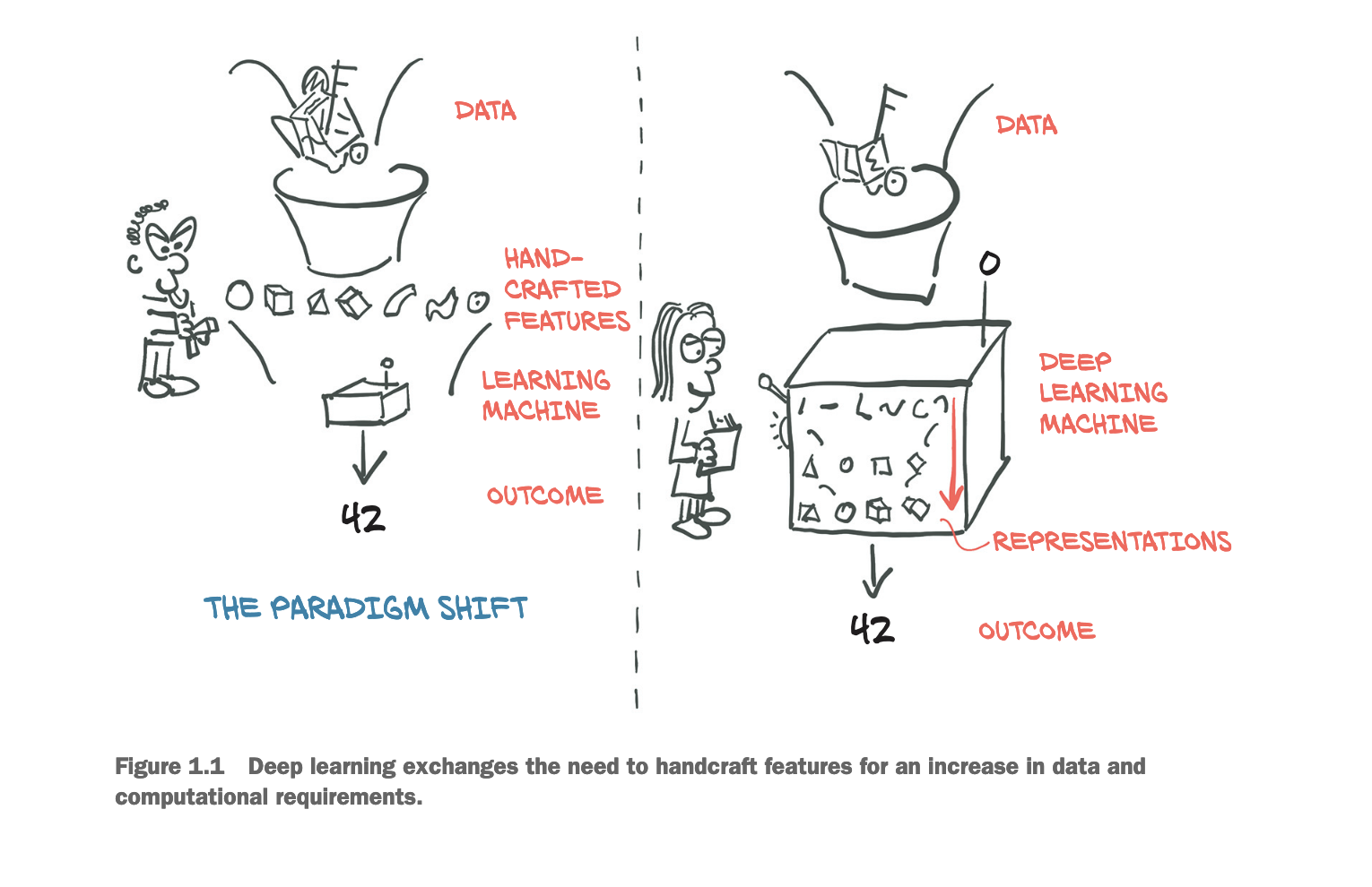
From: Deep Learning with PyTorch
Third, because they are so huge and architecturally complex, LLMs are extremely compute-intensive to train (or pre-train), and because they’re very good at transfer learning (i.e. between machine learning tasks), they’re fairly easy to fine-tune.
So, what are the implications in how we compress now?
We’ve lost fine-grained control over the input data
All of this has had implications for machine learning architectures and economics, the first being that our control of the model has shifted. In order to understand this cycle, we need to understand a bit about internet history.
The early history of computing – and machine learning as a subset – was built on mainframes, which are enormous data servers that processed and kept track of data they generated in isolation from each other. In the 1970s, university researchers started configuring these standalone machines to talk to one another. ARPANET could be seen as the predecessor of the Internet. Here’s what researchers at the University of Utah wrote in 1970, after connecting the university’s computers to ARPANET:
"We have found that, in the process of connecting machines and operating systems together, a great deal of rapport has been established between personnel at the various network node sites. The resulting mixture of ideas, discussions, disagreements and resolutions, has been highly refreshing and beneficial to all involved, and we regard human interaction as a valuable by-product of the main effect."
When compute moved from machines to the network, the creators of these systems started keeping track of data movement and logging it, to get a consolidated view of data flows across their systems. Companies were already retaining analytical data needed to run critical business operations in relational databases, but access to that data was structured and processed in batch increments on a daily or weekly basis. This new logfile data moved quickly, and with a level of variety absent from traditional databases.
Capturing log data at scale began the rise of the Big Data era, which resulted in a great deal of variety, velocity, and volume of data movements. The Apache Webserver logfile was one of the greatest enablers of Big Data. The rise in data volumes coincided with data storage becoming much cheaper, enabling companies to store everything they collected on racks of commodity hardware.
When the data science boom hit in the early 2010s, the initial focus was on collecting as much data as possible, understanding a company’s datasets and creating models from them.
Once companies realized they sat on potential goldmines of unstructured data – none of which were actionable – they started hiring data scientists to make sense of it all. The practice of modern data science arose from statisticians who observed the amount of data being generated and processed required methods beyond the scope of academic statistics and processing methods on single machines.
At the same time, model artifacts and deliverables moved from pure one-off analyses that lived on individuals’ laptops, to production software such as the services powering web applications like Amazon and Netflix’s recommendations, risk scoring for fraud, and medical diagnostic tools. This software required models be portable, low-latency, and be managed in a central place, which meant building systems and platforms on which to manage them. The term “MLOps” arose to define the boundaries of model management and operationalization.
As Marianne Bellotti describes in “Kill It With Fire, ” software development paradigms are a cycle, a continuous tradeoff between how cheap it is to process data on a single machine versus sending it over the network.
“Technology is, and probably always will be, an expensive element of any organization’s operational model. A great deal of advancement and market co-creation in technology can be understood as the interplay between hardware costs and network costs. Computers are data processors. They move data around and rearrange it into different formats and displays for us. All advancements with data processors come down to one of two things: either you make the machine faster or you make the pipes delivering data faster.”
We started with mainframe processing. Once we broke apart the mainframe into personal computers that were cheaper, we could write code locally. Then, our computers became even smaller and internet bandwidth became cheap, it made more sense to process and develop over the wire, particularly since much of our code was now tied up in web applications that lived in server farms. So, we sent everything to the cloud and started bundling development there.
Now that training is the bottleneck and bandwidth is cheap, we rely on external LLM artifacts that create generalized paradigms of compression not specific to our busines use-cases. We’ve outsourced the model creation to a few large companies (OpenAI, Meta, Mistral, etc.) and these base model artifacts now live either behind an API or are available somewhere like the HuggingFace model hub.
LLM model artifacts right now come in two-ish flavors:
- API-based calls to models hosted with proprietary vendors, most likely OpenAI these days, and with OpenAI-interfacing APIs like Together or using model artifacts hosted on model hubs like HuggingFace
- Using your own trained, or more likely, fine-tuned model artifacts starting with a base model as an API or model hub model on your own public cloud GPU-based instances or in an HPC Slurm-style cluster. This is only now starting to pick up steam in 2024, but I expect it will grow, a lot.
So what we’ve done is changed the amount of the model we have agency over in the tradeoff for more generalizable compression. All of our data now does not live in-house, it only does in the case that we’re fine-tuning it, and even then, we are likely using also at least some public datasets that have been put together specifically for the purporses for fine-tuning.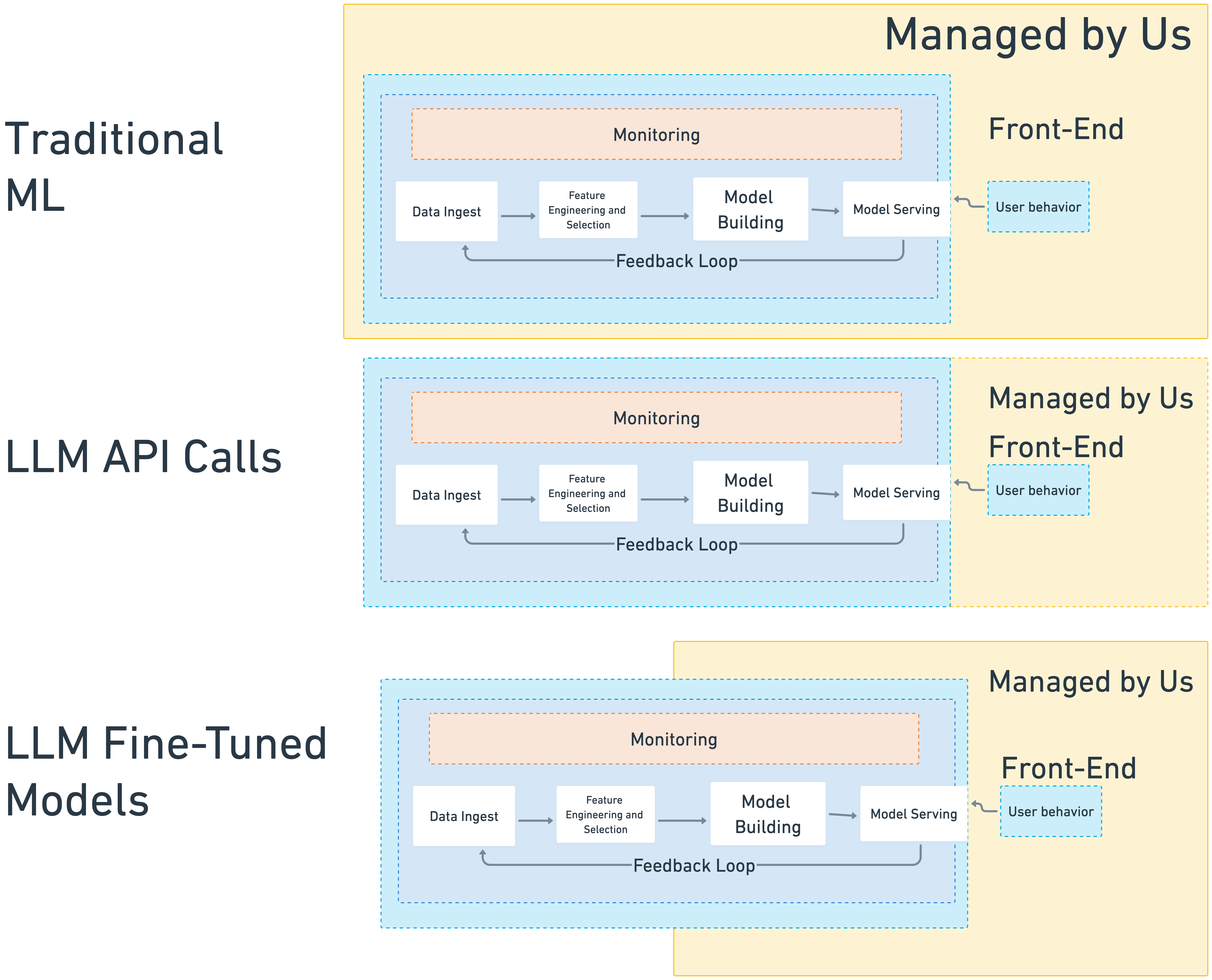
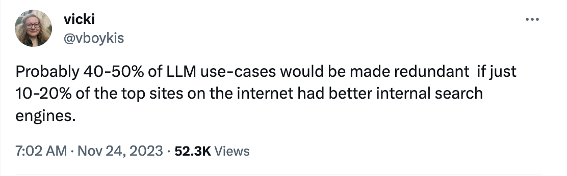
In each of the cases, in gaining a larger amount of compressed data, we give up some degree of internal control over our model state. This is also the reason why RAG as an architecture is so popular. At least 50% of LLM use-cases are straight-up search, because web search (except for Kagi, everyone should use Kagi it’s great) is in a very bad state.
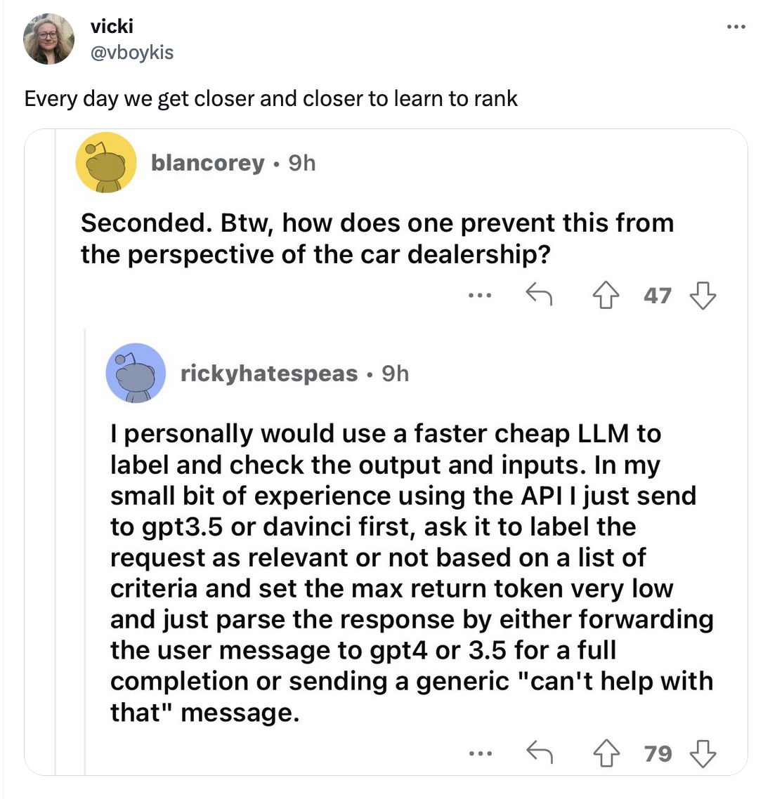
RAG gives us back some control because it allows us to perform the data updates and search fine-tuning we used to in traditional architectures but also combine the strength of the generalist model. In a lot of ways, we are just going back to Learn to Rank, but with less control over the first-pass model.
Textual Features and Metrics and Evaluation
When we evaluated traditional models running either online or offline, we often cared about the traditional metrics: for offline, precision, recall, F1, ROC/AUC. For online, clickthrough rate. For operational, i/o, model artifact response time in milliseconds, and service uptime. As second-level metrics, we often cared about the size of the model artifact in GB, the size of the input data, how long it took to train and re-train the model, and feature completeness (i.e. missing values, imputation, etc.)
Because we are now mostly compressing text rather than numerical or heterogenous features, we suddenly care about also the things above, but a lot of new text-based metrics specific to models whose goal is to complete strings of text. We are now extremely concerned with how strings perform at scale, reading strings, writing strings, and calculating probabilities of returning specific strings from the model.
Specific examples include “time to first token”, tokens per second (the ultimate metric), and understanding and evaluating logprobs.
GPU Architectures
Finally, this entire new landscape necessitates new training and serving frameworks. The size of the models and the specific computational power they need mean suddenly GPUs come into the mix. GPUs are, needless to say, different beasts. In many of our earlier architectures we spent a lot of time in the in/out of our preprocessing data pipelines. To solve the complex problems of coordination, analysis, and engineering that machine learning in production involves, many companies and teams worked on in-house platform approaches which were open-sourced as top-level Apache projects, or turned into tools built by vendors.
Examples in the ML ecosystem are:
Apache Spark: a distributed batch computational platform processing large quantities of data that’s still widely used today

Apache Airflow: a scheduler for data engineering pipelines and data orchestration

Apache Lucene: a search engine. Elasticsearch is one of the most popular distributed and horizontally scalable search frameworks built on top of Apache Lucene.
Many of these tools were built under the assumptions of: we need to coordinate lots of small pieces of log data flowing from our app’s usage servers into a place where it can be aggregated for modeling, so we care about coordination of distributed systems.
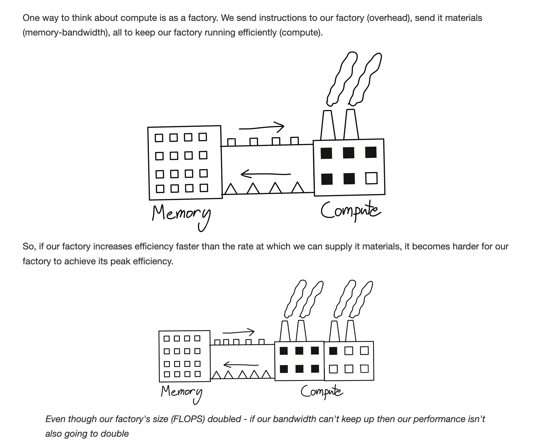
In the world of GPU training and serving, we now have a different problem. We need to get everything onto the GPU as fast as possible so we can process it, because it’s inefficient to have the GPU idling, waiting for more data operations.
As a result, it makes sense to have special GPU clusters that we now need to manage with specific considerations.
TL; DR
There is a lot more we can write for each of these categories and I hope to dive deeper on some of them in future posts. The bottom line is that a lot has changed in leading-edge ML applications over the past year as we’ve moved compression from inside our enterprises to the internet at large.
We’ve moved from smaller, business-specific models that perform specific tasks, to very large, generalist models that do one thing: text completion. Around these new models, we have a new set of metrics and operational and infrastructure concerns, particularly if we are using them as model artifacts (versus APIs). The interesting thing is that, now that we’ve shifted from small to big, the pendulum is again shifting to smaller models that people are starting to fine-tune and run on their own, which will likely make everything I’ve written here out of date in a month or two. One thing that remains constant is that we are still performing compression. The question is, where, and how much do we control it.