GGUF, the long way around

Table of Contents
- How We Use LLM Artifacts
- What is a machine learning model
- Writing the model code
- What is a file
- How does PyTorch write objects to files?
- Conclusion
How We Use LLM Artifacts
Large language models today are consumed in one of several ways:
- As API endpoints for proprietary models hosted by OpenAI, Anthropic, or major cloud providers
- As model artifacts downloaded from HuggingFace’s Model Hub and/or trained/fine-tuned using HuggingFace libraries and hosted on local storage
- As model artifacts available in a format optimized for local inference, typically GGUF, and accessed via applications like
llama.cpporollama - As ONNX, a format which optimizes sharing between backend ML frameworks
For a side project, I’m using llama.cpp, a C/C++-based LLM inference engine targeting M-series GPUs on Apple Silicon.
When running llama.cpp, you get a long log that consists primarily of key-value pairs of metadata about your model architecture and then its performance (and no yapping).
make -j && ./main -m /Users/vicki/llama.cpp/models/mistral-7b-instruct-v0.2.Q8_0.gguf -p "What is Sanremo? no yapping"

Sanremo Music Festival (Festival di Sanremo) is an annual Italian music competition held in the city of Sanremo since 1951. It's considered one of the most prestigious and influential events in the Italian music scene. The festival features both newcomers and established artists competing for various awards, including the Big Award (Gran Premio), which grants the winner the right to represent Italy in the Eurovision Song Contest. The event consists of several live shows where artists perform their original songs, and a jury composed of musicians, critics, and the public determines the winners through a combination of points. [end of text]

llama_print_timings:        load time =   11059.32 ms
llama_print_timings:      sample time =      11.62 ms /   140 runs   (    0.08 ms per token, 12043.01 tokens per second)
llama_print_timings: prompt eval time =      87.81 ms /    10 tokens (    8.78 ms per token,   113.88 tokens per second)
llama_print_timings:        eval time =    3605.10 ms /   139 runs   (   25.94 ms per token,    38.56 tokens per second)
llama_print_timings:       total time =    3730.78 ms /   149 tokens
ggml_metal_free: deallocating
Log end
These logs can be found in the Llama.cpp codebase. There, you’ll also find GGUF. GGUF (GPT-Generated Unified Format) is the file format used to serve models on Llama.cpp and other local runners like Llamafile, Ollama and GPT4All.
To understand how GGUF works, we need to first take a deep dive into machine learning models and the kinds of artifacts they produce.
What is a machine learning model
Let’s start by describing a machine learning model. At its simplest, a model is a file or a collection of files that contain the model architecture and weights and biases of the model generated from a training loop.
In LLM land, we’re generally interested in transformer-style models and architectures.
In a transformer, we have many moving parts.
- For the input, we use training data corpuses aggregated from human-generated nautural language content
- For the algorithm, we
- Convert that data into embeddings
- Positionally encoding the embeddings to provide information about where the words are in relation to each other in the sequence
- Creating multi-headed self-attention for each word in relation to each other word in the sequence based on an initialized combinations of weights
- Normalize layers via softmax
- Run the resulting matrix through a feedfoward neural network
- Project the output into the correct vector space for the desired task
- Calculate loss and then update model parameters
- The output: Generally for for chat completions tasks, the model returns the statistical likelihood that any given word completes a phrase. It does this again and again for every word in the phrase, because of its autoregressive nature.
If the model is served as a consumer end-product, it only returns the actual text output based on the highest probabilities, with numerous strategies for how that text is selected.
In short, we convert inputs to outputs using an equation. In addition to the model’s output, we also have the model itself that is generated as an artifact of the modeling process.
Starting with a simple model
Let’s take a step back from the complexity of transformers and build a small linear regression model in PyTorch. Lucky for us, linear regression is also a (shallow) neural network, so we can work with it in PyTorch and map our simple model to more complex ones using the same framework.
Linear regression takes a set of numerical inputs and generates a set of numerical outputs. (In contrast to transformers, which take a set of text inputs and generates a set of text inputs and their related numerical probabilities.)
For example, let’s say that we produce artisinal hazlenut spread for statisticians, and want to predict how many jars of Nulltella we’ll produce on any given day. Let’s say we have some data available to us, and that is, how many hours of sunshine we have per day, and how many jars of Nulltella we’ve been able to produce every day.
It turns out that we feel more inspired to produce hazlenut spread when it’s sunny out, and we can clearly see this relationship between input and output in our data (we do not produce Nulltella Friday-Sunday because we prefer to spend those days writing about data serialization formats):
| day_id | hours   | jars |
|--------|---------|------|
| mon    | 1       | 2    |
| tues   | 2       | 4    |
| wed    | 3       | 6    |
| thu    | 4       | 8    |
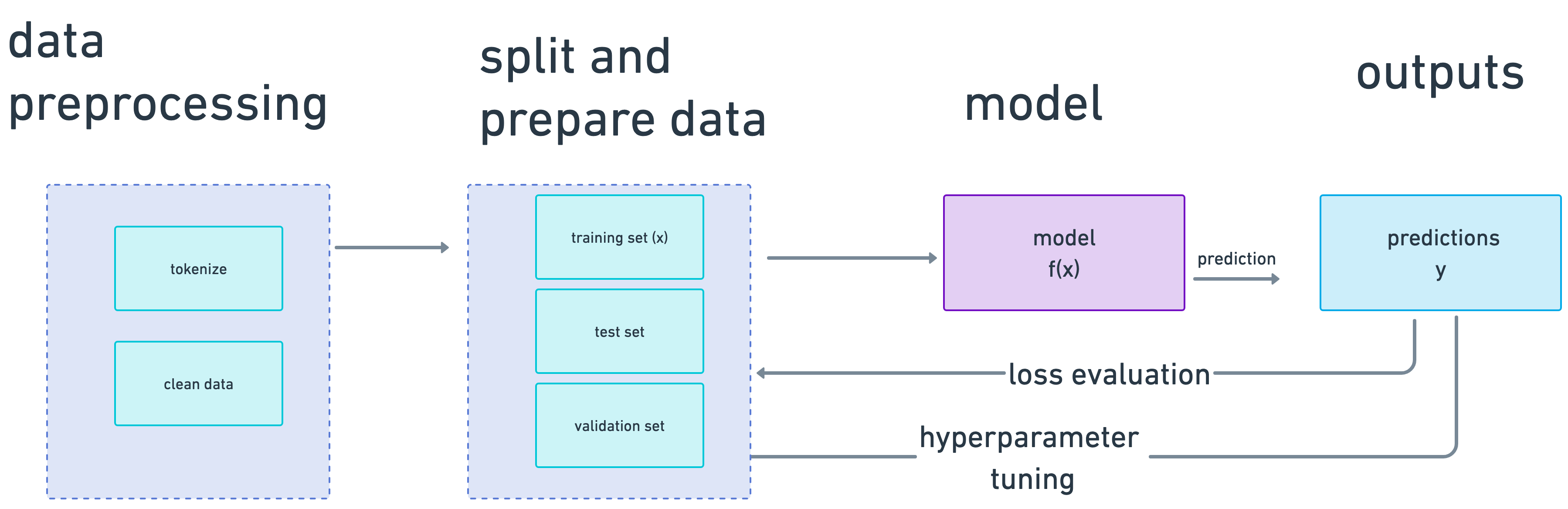
This is the data we’ll use to train our model. We’ll need to split this data into three parts:
- used to train our model (training data)
- used to test the accuracy of our model (test data)
- used to tune our hyperparameters, meta-aspects of our model like the learning rate, (validation set) during the model training phase.
In the specific case of linear regression, there technically are no hyperparameters, although we can plausibly consider the learning rate we set in PyTorch to be one. Let’s assume we have 100 of these data points values.
We split the data into train, test, and validation. A usual accepted split is to use 80% of data for training/validation and 20% for testing. We want our model to have access to as much data as possible so it learns a more accurate representation, so we leave most data for train.
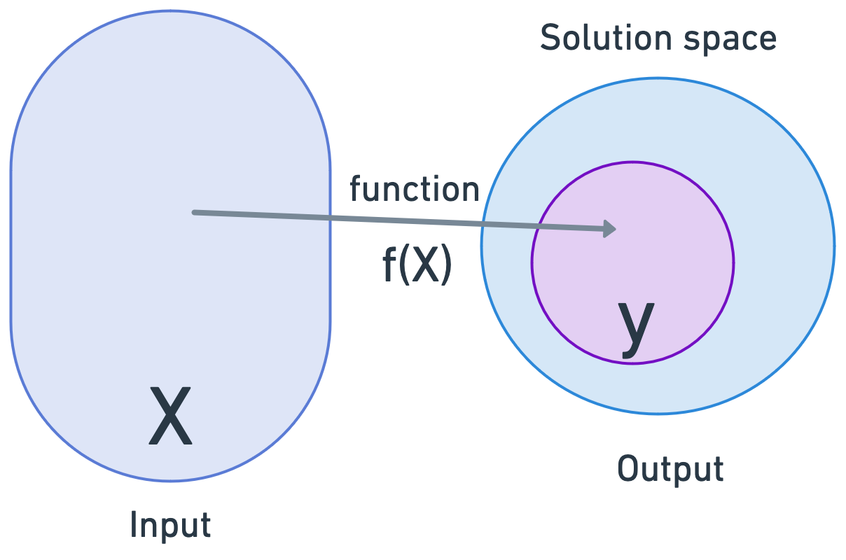
Now that we have our data, we need to write our algorithm. The equation to get output \(Y\) from inputs \(X\) for linear regression is:
$$y = \beta_0 + \beta_1 x_1 + \varepsilon $$
This tells us that the output, \(y\) (the number of jars of Nulltella), can be predicted by:
- \(x_1\) - one input variable (or feature), (hours of sunshine)
- \(\beta_1\) - with its given weight, also called parameters, (how important that feature is)
- plus an error term \(\varepsilon\) that is the difference between the observed and actual values in a population that captures the noise of the model
Our task is to continuously predict and adjust our weights to optimally solve this equation for the difference between our actual \(Y\) as presented by our data and a predicted \(\hat Y\) based on the algorithm to find the smallest sum of squared differences, \(\sqrt{\frac{1}{n} \sum_{i=1}^{n} (y_i - \hat{y}_i)^2}\), between each point and the line. In other words, we’d like to minimize \(\varepsilon\), because it will mean that, at each point, our \(\hat Y\) is as close to our actual \(Y\) as we can get it, given the other points.
We optimize this function through gradient descent, where we start with either zeros or randomly-initialized weights and continue recalculating both the weights and error term until we come to an optimal stopping point. We’ll know we’re succeeding because our loss, as calculated by RMSE should incrementally decrease in every training iteration.
Here’s the whole model learning process end-to-end (with the exception of tokenization, which we only do for models where features are text and we want to do language modeling):
Writing the model code
Now, let’s get more concrete and describe these ideas in code. When we train our model, we initialize our function with a set of feature values.
Let’s add our data into the model by initializing both \(x_1\) and \(Y\) as PyTorch Tensor objects.
# Hours of sunshine
X = torch.tensor([[1.0], [2.0], [3.0], [4.0]], dtype=torch.float32)

# Jars of Nulltella
y = torch.tensor([[2.0], [4.0], [6.0], [8.0]], dtype=torch.float32)
Within code, our input data is X, which is a torch tensor object, and our output data is y. We initialize a LinearRegression which subclasses the PyTorch Module, with one linear layer, which has one input feature (sunshine) and one output feature (jars of Nulltella).
I’m going to include the code for the whole model, and then we’ll talk through it piece by piece.
import torch
import torch.nn as nn
import torch.optim as optim

X = torch.tensor([[1.0], [2.0], [3.0], [4.0]], dtype=torch.float32)
y = torch.tensor([[2.0], [4.0], [6.0], [8.0]], dtype=torch.float32)

# Define a linear regression model and its forward pass
class LinearRegression(nn.Module):
    def __init__(self):
        super(LinearRegression, self).__init__()
        self.linear = nn.Linear(1, 1)  # 1 input feature, 1 output feature

    def forward(self, x):
        return self.linear(x)

# Instantiate the model
model = LinearRegression()

# Inspect the model's state dictionary
print(model.state_dict())

# Define loss function and optimizer
criterion = nn.MSELoss()
# setting our learning rate "hyperparameter" here
optimizer = optim.SGD(model.parameters(), lr=0.01)

# Training loop that includes forward and backward pass
num_epochs = 100
for epoch in range(num_epochs):
    # Forward pass
    outputs = model(X)
    loss = criterion(outputs, y)
    RMSE_loss  = torch.sqrt(loss)

    # Backward pass and optimization
    optimizer.zero_grad()  # Zero out gradients
    RMSE_loss.backward()  # Compute gradients
    optimizer.step()  # Update weights

    # Print progress
    if (epoch+1) % 10 == 0:
        print(f'Epoch [{epoch+1}/{num_epochs}], Loss: {loss.item():.4f}')

# After training, let's test the model
test_input = torch.tensor([[5.0]], dtype=torch.float32)
predicted_output = model(test_input)
print(f'Prediction for input {test_input.item()}: {predicted_output.item()}')
Once we have our input data, we then initialize our model, a LinearRegression which subclasses Module base class specifically for linear regression.
A forward pass involves feeding our data into the neural network and making sure it propogagtes through all the layers. Since we only have one, we have to pass our data to a single linear layer. The forward pass is what calculates our predicted Y.
class LinearRegression(nn.Module):
    def __init__(self):
        super(LinearRegression, self).__init__()
        self.linear = nn.Linear(1, 1)  # 1 input feature, 1 output feature

    def forward(self, x):
        return self.linear(x)
We pick how we’d like to optimize the results of the model, aka how its loss should converge. In this case, we start with mean squared error, and then modify it to use RMSE, the square root of the average squared difference between the predicted values and the actual values in a dataset.
# Define loss function and optimizer
criterion = torch.sqrl(nn.MSELoss())  # RMSE in the training loop
optimizer = optim.SGD(model.parameters(), lr=0.01)

....
for epoch in range(num_epochs):
    # Forward pass
    outputs = model(X)
    loss = criterion(outputs, y)
    RMSE_loss  = torch.sqrt(loss)
Now that we’ve defined how we’d like the model to run, we can instantiate the model object itself:
Instantiating the model object
model = LinearRegression()
print(model.state_dict())
Notice that when we instantiate a nn.Module, it has an attribute called the “state_dict”. This is important. The state dict holds the information about each layer and the parameters in each layer, aka the weights and biases.
At its heart, it’s a Python dictionary.
In this case, the implementation for LinearRegression returns an ordered dict with each layer of the network and values of those layers. Each of the values is a Tensor.
OrderedDict([('linear.weight', tensor([[0.5408]])), ('linear.bias', tensor([-0.8195]))])

for param_tensor in model.state_dict():
    print(param_tensor, "\t", model.state_dict()[param_tensor].size())

linear.weight    torch.Size([1, 1])
linear.bias      torch.Size([1])
For our tiny model, it’s a small OrderedDict of tuples. You can imagine that this collection of tensors becomes extremely large and memory-intensive in a large network such as a transformer. If each parameter (each Tensor object) takes up 2 bytes in memory, a 7-billion parameter model can take up 14GB in GPU.
We then run the forward and backward passes for the model in loops. In each step, we do a forward pass to perform the calculation, a backward pass to update the weights of our model object, and then we add all that information to our model parameters.
# Define loss function and optimizer
criterion = nn.MSELoss()
optimizer = optim.SGD(model.parameters(), lr=0.01)

# Training loop
num_epochs = 100
for epoch in range(num_epochs):
    # Forward pass
    outputs = model(X)
    loss = criterion(outputs, y)
    RMSE_loss  = torch.sqrt(loss)

    # Backward pass and optimization
    optimizer.zero_grad()  # Zero out gradients
    RMSE_loss.backward()  # Compute gradients
    optimizer.step()  # Update weights

    # Print progress
    if (epoch+1) % 10 == 0:
        print(f'Epoch [{epoch+1}/{num_epochs}], Loss: {loss.item():.4f}')
Once we’ve completed these loops, we’ve trained the model artifact. What we now have once we have trained a model is an in-memory object that represents the weights, biases, and metadata of that model, stored within our instance of our LinearRegression module.
As we run the training loop, we can see our loss shrink. That is, the actual values are getting closer to the predicted:
Epoch [10/100], Loss: 33.0142
Epoch [20/100], Loss: 24.2189
Epoch [30/100], Loss: 16.8170
Epoch [40/100], Loss: 10.8076
Epoch [50/100], Loss: 6.1890
Epoch [60/100], Loss: 2.9560
Epoch [70/100], Loss: 1.0853
Epoch [80/100], Loss: 0.4145
Epoch [90/100], Loss: 0.3178
Epoch [100/100], Loss: 0.2974
We can also see if we print out the state_dict that the parameters have changed as we’ve computed the gradients and updated the weights in the backward pass:
"""before"""
OrderedDict([('linear.weight', tensor([[-0.6216]])), ('linear.bias', tensor([0.7633]))])
linear.weight    torch.Size([1, 1])
linear.bias      torch.Size([1])
{'state': {}, 'param_groups': [{'lr': 0.01, 'momentum': 0, 'dampening': 0, 'weight_decay': 0, 'nesterov': False, 'maximize': False, 'foreach': None, 'differentiable': False, 'params': [0, 1]}]}
Epoch [10/100], Loss: 33.0142
Epoch [20/100], Loss: 24.2189
Epoch [30/100], Loss: 16.8170
Epoch [40/100], Loss: 10.8076
Epoch [50/100], Loss: 6.1890
Epoch [60/100], Loss: 2.9560
Epoch [70/100], Loss: 1.0853
Epoch [80/100], Loss: 0.4145
Epoch [90/100], Loss: 0.3178
Epoch [100/100], Loss: 0.2974

"""after"""
OrderedDict([('linear.weight', tensor([[1.5441]])), ('linear.bias', tensor([1.3291]))])
The optimizer, as we see, has its own state_dict, which consists of these hyperparameters we discussed before: the learning rate, the weight decay, and more:
print(optimizer.state_dict())
{'state': {}, 'param_groups': [{'lr': 0.01, 'momentum': 0, 'dampening': 0, 'weight_decay': 0, 'nesterov': False, 'maximize': False, 'foreach': None, 'differentiable': False, 'params': [0, 1]}]}
Now that we have a trained model object, we can pass in new feature values for the model to evaluate. For example we can pass in an X value of 5 hours of sunshine and see how many jars of Nulltella we expect to make.
We do this by passing in 5 to the instantiated model object, which is now a combination of the method used to run the linear regression equation and our state dict, the weights, the current set of weights and biases to give a new predicted value. We get 9 jars, which pretty close to what we’d expect.
test_input = torch.tensor([[5.0]], dtype=torch.float32)
predicted_output = model(test_input)
print(f'Prediction for input {test_input.item()}: {predicted_output.item()}')
Prediction for input 5.0: 9.049455642700195
I’m abstracting away an enormous amount of detail for the sake of clarity, namely the massive amount of work PyTorch does in moving this data in and out of GPUs and working with GPU-efficient datatypes for efficient computing which is a large part of the work of the library. We’ll skip these for now for simplicity.
Serializing our objects
So far, so good. We now have stateful Python objects in-memory that convey the state of our model. But what happens when we need to persist this very large model, that we likely spent 24+ hours training, and use it again?
This scenario is described here,
Suppose a researcher is experimenting with a new deep-learning model architecture, or a variation on an existing one. Her architecture is going to have a whole bunch of configuration options and hyperparameters: the number of layers, the types of each layers, the dimensionality of various vectors, where and how to normalize activations, which nonlinearity(ies) to use, and so on. Many of the model components will be standard layers provided by the ML framework, but the researcher will be inserting bits and pieces of novel logic as well.
Our researcher needs a way to describe a particular concrete model – a specific combination of these settings – which can be serialized and then reloaded later. She needs this for a few related reasons:
She likely has access to a compute cluster containing GPUs or other accelerators she can use to run jobs. She needs a way to submit a model description to code running on that cluster so it can run her model on the cluster.
While those models are training, she needs to save snapshots of their progress in such a way that they can be reloaded and resumed, in case the hardware fails or the job is preempted. Once models are trained, the researcher will want to load them again (potentially both a final snapshot, and some of the partially-trained checkpoints) in order to run evaluations and experiments on them.
What do we mean by serialization? It’s the process of writing objects and classes from our programming runtime to a file. Deserialization is the process of converting data on disk to programming language objects in memory. We now need to seralize the data into a bytestream that we can write to a file.

Why “serialization”? Because back in the Old Days, data used to be stored on tape, which required bits to be in order sequentially on tape.
Since many transformer-style models are trained using PyTorch these days, artifacts use PyTorch’s save implementation for serializing objects to disk.
What is a file
Again, let’s abstract away the GPU for simplicity and assume we’re performing all these computations in CPU. Python objects live in memory. This memory is allocated in a special private heap at the beginning of their lifecycle, in private heap managed by the Python memory manager, with specialized heaps for different object types.
When we initialize our PyTorch model object, the operating system allocates memory through lower-level C functions, namely malloc, via default memory allocators.
When we run our code with tracemalloc, we can see how memory for PyTorch is actually allocated on CPU (keep in mind that, again, GPU operations are completely different).
import tracemalloc

tracemalloc.start()

.....
pytorch
...

snapshot = tracemalloc.take_snapshot()
top_stats = snapshot.statistics('lineno')

print("[ Top 10 ]")
for stat in top_stats[:10]:
    print(stat)

[ Top 10 ]
<frozen importlib._bootstrap_external>:672: size=21.1 MiB, count=170937, average=130 B
/Users/vicki/.pyenv/versions/3.10.0/lib/python3.10/inspect.py:2156: size=577 KiB, count=16, average=36.0 KiB
/Users/vicki/.pyenv/versions/3.10.0/lib/python3.10/site-packages/torch/_dynamo/allowed_functions.py:71: size=512 KiB, count=3, average=171 KiB
/Users/vicki/.pyenv/versions/3.10.0/lib/python3.10/dataclasses.py:434: size=410 KiB, count=4691, average=90 B
/Users/vicki/.pyenv/versions/3.10.0/lib/python3.10/site-packages/torch/_dynamo/allowed_functions.py:368: size=391 KiB, count=7122, average=56 B
/Users/vicki/.pyenv/versions/3.10.0/lib/python3.10/site-packages/torch/_dynamo/allowed_functions.py:397: size=349 KiB, count=1237, average=289 B
<frozen importlib._bootstrap_external>:128: size=213 KiB, count=1390, average=157 B
/Users/vicki/.pyenv/versions/3.10.0/lib/python3.10/functools.py:58: size=194 KiB, count=2554, average=78 B
/Users/vicki/.pyenv/versions/3.10.0/lib/python3.10/site-packages/torch/_dynamo/allowed_functions.py:373: size=136 KiB, count=2540, average=55 B
<frozen importlib._bootstrap_external>:1607: size=127 KiB, count=1133, average=115 B
Here, we can see we imported 170k objects from imports, and that the rest of the allocation came from allowed_functions in torch.
How does PyTorch write objects to files?
We can also more explicitly see the types of these objects in memory. Among all the other objects created by PyTorch and Python system libraries, we can see our Linear object here, which has state_dict as a property. We need to serialize this object into a bytestream so we can write it to disk.
import gc
# Get all live objects
all_objects = gc.get_objects()

# Extract distinct object types
distinct_types = set(type(obj) for obj in all_objects)

# Print distinct object types
for obj_type in distinct_types:
    print(obj_type.__name__)

InputKind
KeyedRef
ReLU
Manager
_Call
UUID
Pow
Softmax
Options
_Environ
**Linear**
CFunctionType
SafeUUID
_Real
JSONDecoder
StmtBuilder
OutDtypeOperator
MatMult
attrge
PyTorch serializes objects to disk using Python’s pickle framework and wrapping the pickle load and dump methods.
Pickle traverses the object’s inheritance hierarchy and converts each object encountered into streamable artifacts. It does this recursively for nested representations (for example, understanding nn.Module and Linear inheriting from nn.Module) and converting these representations to byte representations so that they can be written to file.
As an example, let’s take a simple function and write it to a pickle file.
import torch.nn as nn
import torch.optim as optim
import pickle

X = torch.tensor([[1.0], [2.0], [3.0], [4.0]], dtype=torch.float32)

with open('tensors.pkl', 'wb') as f:
    pickle.dump(X, f)
when we inspect the pickled object with pickletools, we get an idea of how the data is organized.
We import some functions that load the data as a tensor, then the actual storage of that data, then its type. The module does the inverse when converting from pickle files to Python objects.
python -m pickletools tensors.pkl
    0: \x80 PROTO      4
    2: \x95 FRAME      398
   11: \x8c SHORT_BINUNICODE 'torch._utils'
   25: \x94 MEMOIZE    (as 0)
   26: \x8c SHORT_BINUNICODE '_rebuild_tensor_v2'
   46: \x94 MEMOIZE    (as 1)
   47: \x93 STACK_GLOBAL
   48: \x94 MEMOIZE    (as 2)
   49: (    MARK
   50: \x8c     SHORT_BINUNICODE 'torch.storage'
   65: \x94     MEMOIZE    (as 3)
   66: \x8c     SHORT_BINUNICODE '_load_from_bytes'
   84: \x94     MEMOIZE    (as 4)
   85: \x93     STACK_GLOBAL
   86: \x94     MEMOIZE    (as 5)
   87: B        BINBYTES   b'\x80\x02\x8a\nl\xfc\x9cF\xf9 j\xa8P\x19.\x80\x02M\xe9\x03.\x80\x02}q\x00(X\x10\x00\x00\x00protocol_versionq\x01M\xe9\x03X\r\x00\x00\x00little_endianq\x02\x88X\n\x00\x00\x00type_sizesq\x03}q\x04(X\x05\x00\x00\x00shortq\x05K\x02X\x03\x00\x00\x00intq\x06K\x04X\x04\x00\x00\x00longq\x07K\x04uu.\x80\x02(X\x07\x00\x00\x00storageq\x00ctorch\nFloatStorage\nq\x01X\n\x00\x00\x006061074080q\x02X\x03\x00\x00\x00cpuq\x03K\x04Ntq\x04Q.\x80\x02]q\x00X\n\x00\x00\x006061074080q\x01a.\x04\x00\x00\x00\x00\x00\x00\x00\x00\x00\x80?\x00\x00\x00@\x00\x00@@\x00\x00\x80@'
  351: \x94     MEMOIZE    (as 6)
  352: \x85     TUPLE1
  353: \x94     MEMOIZE    (as 7)
  354: R        REDUCE
  355: \x94     MEMOIZE    (as 8)
  356: K        BININT1    0
  358: K        BININT1    4
  360: K        BININT1    1
  362: \x86     TUPLE2
  363: \x94     MEMOIZE    (as 9)
  364: K        BININT1    1
  366: K        BININT1    1
  368: \x86     TUPLE2
  369: \x94     MEMOIZE    (as 10)
  370: \x89     NEWFALSE
  371: \x8c     SHORT_BINUNICODE 'collections'
  384: \x94     MEMOIZE    (as 11)
  385: \x8c     SHORT_BINUNICODE 'OrderedDict'
  398: \x94     MEMOIZE    (as 12)
  399: \x93     STACK_GLOBAL
  400: \x94     MEMOIZE    (as 13)
  401: )        EMPTY_TUPLE
  402: R        REDUCE
  403: \x94     MEMOIZE    (as 14)
  404: t        TUPLE      (MARK at 49)
  405: \x94 MEMOIZE    (as 15)
  406: R    REDUCE
  407: \x94 MEMOIZE    (as 16)
  408: .    STOP
highest protocol among opcodes = 4
The main issue with pickle as a file format is that it not only bundles executable code, but that there are no checks on the code being read, and without schema guarantees, you can pass something to the pickle that’s malicious,
The insecurity is not because pickles contain code, but because they create objects by calling constructors named in the pickle. Any callable can be used in place of your class name to construct objects. Malicious pickles will use other Python callables as the “constructors.” For example, instead of executing “models.MyObject(17)”, a dangerous pickle might execute “os.system(‘rm -rf /’)”. The unpickler can’t tell the difference between “models.MyObject” and “os.system”. Both are names it can resolve, producing something it can call. The unpickler executes either of them as directed by the pickle.'
How Pickle works
Pickle initially worked for Pytorch-based models because it was also closely coupled to the Python ecosystem and initial ML library artifacts were not the key outputs of deep learning systems.
The primary output of research is knowledge, not software artifacts. Research teams write software to answer research questions and improve their/their team’s/their field’s understanding of a domain, more so than they write software in order to have software tools or solutions.
However, as the use of transformer-based models picked up after the release of the Transformer paper in 2017, so did the use of the transformers library, which delegates the load call to PyTorch’s load methods, which uses pickle.
Once practitioners started creating and uploading pickled model artifacts to model hubs like HuggingFace, machine learning model supply chain security became an issue.
From pickle to safetensors
As machine learning with deep learning models trained with PyTorch exploded, these security issues came to a head, and in 2021, Trail of Bits released a post the insecurity of pickle files.
Engineers at HuggingFace started developing a library known as safetensors as an alternative to pickle. Safetensors was a developed to be efficient, but, also safer and more ergonomic than pickle.
First, safetensors is not bound to Python as closely as Pickle: with pickle, you can only read or write files in Python. Safetensors is compatible across languages. Second, safetensors also limits language execution, functionality available on serialization and deserialization. Third, because the backend of safetensors is written in Rust, it enforces type safety more rigorously. Finally, safetensors was optimized for work specifically with tensors as a datatype in a way that Pickle was not. That, combined with the fact that it was wirtten in Rust makes it really fast for reads and writes.
After a concerted push from both Trail of Bits and EleutherAI, a security audit of safetensors was conducted and found satisfactory, which led to HuggingFace adapting it as the default format for models on the Hub. going forward. (Big thanks to Stella and Suha for this history and context, and to everyone who contributed to the Twitter thread.)
How safetensors works
How does the safetensors format work? As with most things in LLMs at the bleeding edge, the code and commit history will do most of the talking. Let’s take a look at the file spec.
- 8 bytes: N, an unsigned little-endian 64-bit integer, containing the size of the header
- N bytes: a JSON UTF-8 string representing the header. The header data MUST begin with a { character (0x7B). The header data MAY be trailing padded with whitespace (0x20). The header is a dict like {“TENSOR_NAME”: {“dtype”: “F16”, “shape”: [1, 16, 256], “data_offsets”: [BEGIN, END]}, “NEXT_TENSOR_NAME”: {…}, …}, data_offsets point to the tensor data relative to the beginning of the byte buffer (i.e. not an absolute position in the file), with BEGIN as the starting offset and END as the one-past offset (so total tensor byte size = END - BEGIN). A special key metadata is allowed to contain free form string-to-string map. Arbitrary JSON is not allowed, all values must be strings.
- Rest of the file: byte-buffer.
This is different than state_dict and pickle file specifications, but the addition of safetensors follows the natural evolution from Python objects, to full-fledged file format.
A file is a way of storing our data generated from programming language objects, in bytes on disk. In looking at different file format specs (Arrow,Parquet, protobuf), we’ll start to notice some patterns around how they’re laid out.
- In the file, we need some indicator that this is a type of file “X”. Usually this is represented by a magic byte.
- Then, there is a header that represents the metadata of the file (In the case of machine learning, how many layers we have, the learning rate, and other aspects. )
- The actual data. (In the case of machine learning files, the tensors)
- We then need a spec that tells us what to expect in a file as we read it and what kinds of data types are in the file and how they’re represented as bytes. Essentially, documentation for the file’s layout and API so that we can program a file reader against it.
- One feature the file spec usually tells us is whether data is little or big-endian, that is - whether we store the largest number first or last. This becomes important as we expect files to be read on systems with different default byte layouts.
- We then implement code that reads and writes to that filespec specifically.
One thing we start to notice from having looked at statedicts and pickle files before, is that machine learning data storage follow a pattern: we need to store:
- a large collection of vectors,
- metadata about those vectors and
- hyperparameters
We then need to be able to instantiate model objects that we can hydrate (fill) with that data and run model operations on.
As an example for safetensors from the documentation: We start with a Python dictionary, aka a state dict, save, and load the file.
import torch
from safetensors import safe_open
from safetensors.torch import save_file

tensors = {
   "weight1": torch.zeros((1024, 1024)),
   "weight2": torch.zeros((1024, 1024))
}
save_file(tensors, "model.safetensors")

tensors = {}
with safe_open("model.safetensors", framework="pt", device="cpu") as f:
   for key in f.keys():
       tensors[key] = f.get_tensor(key)
we use the save_file(model.state_dict(), ‘my_model.st’) method to render the file to safetensors
In the conversion process from pickle to safetensors, we also start with the state dict.
Safetensors quickly became the leading format for sharing model weights and architectures to use in further fine-tuning, and in some cases, inference
Checkpoint files
We’ve so far taken a look at simple state_dict files and single safetensors files. But if you’re training a long-running model, you’ll likely have more than just weights and biases to save, and you want to save your state every so often so you can revert if you start to see issues in your trianing run. PyTorch has checkpoints. A checkpoint is a file that has a model state_dict, but also
the optimizer’s state_dict, as this contains buffers and parameters that are updated as the model trains. Other items that you may want to save are the epoch you left off on, the latest recorded training loss, external torch.nn.Embedding layers, and more. This is also saved as a Dictionary and pickled, then unpickled when you need it. All of this is also saved to a dictionary, the
optimizer_state_dict, distinct from themodel_state_dict.
# Additional information
EPOCH = 5
PATH = "model.pt"
LOSS = 0.4

torch.save({
            'epoch': EPOCH,
            'model_state_dict': net.state_dict(),
            'optimizer_state_dict': optimizer.state_dict(),
            'loss': LOSS,
            }, PATH)
In addition, most large language models also now include accompanying files like tokenizers, and on HuggingFace, metadata, etc. So if you’re working with PyTorch models as artifacts generated via the Transformers library, you’ll get a repo that looks like this.
GGML
As work to migrate from pickle to safetensors was ongoing for generalized model fine-tuning and inference, Apple Silicon continued to get a lot better.. As a result, people started bringing modeling work and inference from large GPU-based computing clusters, to local and on-edge devices.
Georgi Gerganov’s project to make OpenAI’s Whisper run locally with Whisper.cpp. was a success and the catalyst for later projects. The combination of the release of Llama-2 as a mostly open-source model, combined with the rise of model compression techniques like LoRA, large language models, which were typically only accessible on lab or industry-grade GPU hardware (inspie of the small CPU-based examples we’ve run here), also acted as a catalyst for thinking about working with and running personalized models locally.
Based on the interest and success of whisper.cpp, Gerganov created llama.cpp, a package for working with Llama model weights, originaly in pickle format, in GGML format, for local inference.
GGML was initialy both a library and a complementary format created specifically for on-edge inference for whisper. You can also perform fine-tuning with it, but generally it’s used to read models trained on PyTorch in GPU Linux-based environments and converted to GGML to run on Apple Silicon.
As an example, here is script for GGML which converts PyTorch GPT-2 checkpoints to the correct format, read as a .bin file.. The files are downloaded from OpenAI.
The resulting GGML file compresses all of these into one and contains:
a magic number with an optional version number
model-specific hyperparameters, including metadata about the model, such as the number of layers, the number of heads, etc. a ftype that describes the type of the majority of the tensors, for GGML files, the quantization version is encoded in the ftype divided by 1000
an embedded vocabulary, which is a list of strings with length prepended.
finally, a list of tensors with their length-prepended name, type, and tensor data
There are several elements that make GGML more efficient for local inference than checkpoint files. First, it makes use of 16-bit floating point representations of model weights. Generally, torch initializes floating point datatypes in 32-bit floats by default. 16-bit, or half precision means that model weights use 50% less memory at compute and inference time without significant loss in model accuracy. Other architectural choices include using C, which offers more efficient memory allocation than Python. And finally, GGML was built optimized for Silicon.
Unfortunately, in its move to efficiency, GGML contained a number of breaking changes that created issues for users.
The largest one was that, since everything, both data and metadata and hyperparameters, was written into the same file, if a model added hyperparameters, it would break backward compatibility that the new file couldn’t pick up. Additionally, no model architecture metadata is present in the file, and each architecture required its own conversion script. All of this led to brittle performance and the creation of GGUF.
Finally, GGUF
GGUF has the same type of layout as GGML, with metadata and tensor data in a single file, but in addition is also designed to be backwards-compatible. The key difference is that previously instead of a list of values for the hyperparameters, the new file format uses a key-value lookup tables which accomodate shifting values.
The intiution we spent building up around how machine learning models work and file formats are laid out now allows us to understand the GGUF format.
First, we know that GGUF models are little-endian by default for specific architectures, which we remember is when the least significant bytes come first and is optimized for different computer hardware architectures.
Then, we have gguf_header_t, which is the header
It includes the magic byte that tells us this is a GGUF file:
Must be `GGUF` at the byte level: `0x47` `0x47` `0x55` `0x46`.
as well as the key-value pairs:
// The metadata key-value pairs.
    gguf_metadata_kv_t metadata_kv[metadata_kv_count];
This file format also offers versioning, in this case we see this is version 3 of the file format.
// Must be `3` for version described in this spec, which introduces big-endian support.
    //
    // This version should only be increased for structural changes to the format.
Then, we have the tensors
gguf_tensor_info_t
The entire file looks like this, and when we work with readers like llama.cpp and ollama, they take this spec and write code to open these files and read them.

Conclusion
We’ve been on a whirlwind adventure to build up our intuition of how machine learning models work, what artifacts they produce, how the machine learning artifact storage story has changed over the past couple years, and finally ended up in GGUF’s documentation to better understand the log that is presented to us when we perform local inference on artifacts in GGUF. Hope this is helpful, and good luck!